Optimal Bounds between f -Divergences and Integral Probability - PowerPoint PPT Presentation
Optimal Bounds between f -Divergences and Integral Probability Metrics Rohit Agrawal (Harvard) Thibaut Horel (MIT) Motivation Is the empirical distribution approximately normal? What is the normal distribution best approximating it? 1 1.0
Optimal Bounds between f -Divergences and Integral Probability Metrics Rohit Agrawal (Harvard) Thibaut Horel (MIT)
Motivation Is the empirical distribution approximately normal? What is the normal distribution best approximating it? 1 1.0 Empirial dist. Normal dist. 0.8 0.6 x ) P ( X 0.4 0.2 0.0 40 20 0 20 40 x
Motivation Is the empirical distribution approximately normal? What is the normal distribution best approximating it? 1 1.0 Empirial dist. Normal dist. 0.8 0.6 x ) P ( X 0.4 0.2 0.0 40 20 0 20 40 x
Motivation Typical learning procedure: ? X Y Problem: what statistical guarantees are implied by maximum likelihood estimation X Y is the Kullback–Leibler divergence Example: if solve 2 observations X given model class M min Y ∈M D( X � Y ) cost function D( ·�· ) Y X
Motivation observations X ? X Y Problem: what statistical guarantees are implied by solve Typical learning procedure: 2 given model class M min Y ∈M D( X � Y ) cost function D( ·�· ) Y X Example: if D( X � Y ) is the Kullback–Leibler divergence ⇒ maximum likelihood estimation
Motivation observations X solve Typical learning procedure: 2 given model class M min Y ∈M D( X � Y ) cost function D( ·�· ) Y X Example: if D( X � Y ) is the Kullback–Leibler divergence ⇒ maximum likelihood estimation Problem: what statistical guarantees are implied by D( X � Y ) ≤ ε ?
Measures of similarity for random variables Ex: Kullback–Leibler (KL) div., mean discrepancy, etc. Ex: total variation dist., max. integral probability metrics How “close” to each other are X and Y ? 3 φ -divergences � � P [ X = y ] �� � � d F ( X , Y ) = sup � E [ f ( X )] − E [ f ( Y )] D φ ( X � Y ) = E y ∼ Y φ � P [ Y = y ] f ∈F for convex φ with φ ( 1 ) = 0 class F of “test” functions χ 2 -div., Hellinger dist., α -div., etc.
4 What is the best lower bound of D φ ( X � Y ) in terms of E [ f ( X )] − E [ f ( Y )] ?
Ex: for the KL divergence, K f Y is the log moment-generating function Result Theorem (Informal) inducing a correspondence between for all X and 5 There exists an explicit function K f ( Y ) : R → R associated with f ( Y ) � � 1. lower bounds D φ ( X � Y ) ≥ L E [ f ( X )] − E [ f ( Y )] 2. upper bounds K f ( Y ) ( t ) ≤ B ( t ) for all t ∈ R
Result Theorem (Informal) inducing a correspondence between for all X and 5 There exists an explicit function K f ( Y ) : R → R associated with f ( Y ) � � 1. lower bounds D φ ( X � Y ) ≥ L E [ f ( X )] − E [ f ( Y )] 2. upper bounds K f ( Y ) ( t ) ≤ B ( t ) for all t ∈ R Ex: for the KL divergence, K f ( Y ) is the log moment-generating function
K f Y t Cumulant-generating function x f Y t e t f Y • we recover the (centered) cumulant-generating function 1 e y y • x and: x 6 Example: for the KL divergence, For a given φ -divergence, defjne: • the convex conjugate φ ⋆ ( y ) = sup x ≥ 0 � � x · y − φ ( x ) • the φ -cumulant-generating function of f ( Y ) � φ ⋆ ( t · f ( Y ) + λ ) − t · f ( Y ) − λ � K f ( Y ) ( t ) = inf λ ∈ R E
Cumulant-generating function • we recover the (centered) cumulant-generating function 6 For a given φ -divergence, defjne: • the convex conjugate φ ⋆ ( y ) = sup x ≥ 0 � � x · y − φ ( x ) • the φ -cumulant-generating function of f ( Y ) � φ ⋆ ( t · f ( Y ) + λ ) − t · f ( Y ) − λ � K f ( Y ) ( t ) = inf λ ∈ R E Example: for the KL divergence, φ ( x ) = x log x and: • φ ⋆ ( y ) = e y − 1 � e t · f ( Y ) − t · E [ f ( Y )] � K f ( Y ) ( t ) = log E
Result where X Y representations of Key technique: use convex analysis to obtain variational Theorem 7 The following are equivalent: for all X 1. K f ( Y ) ( t ) ≤ B ( t ) for all t ∈ R 2. D φ ( X � Y ) ≥ B ⋆ � � E [ f ( X )] − E [ f ( Y )] � φ ⋆ ( t · f ( Y ) + λ ) − t · f ( Y ) − λ � K f ( Y ) ( t ) = inf λ ∈ R E and ⋆ denotes the convex conjugate
Result for all X Key technique: use convex analysis to obtain variational Theorem where 7 The following are equivalent: 1. K f ( Y ) ( t ) ≤ B ( t ) for all t ∈ R 2. D φ ( X � Y ) ≥ B ⋆ � � E [ f ( X )] − E [ f ( Y )] � φ ⋆ ( t · f ( Y ) + λ ) − t · f ( Y ) − λ � K f ( Y ) ( t ) = inf λ ∈ R E and ⋆ denotes the convex conjugate representations of D φ ( X � Y )
3. Negative result, when Applications and examples 2. “Pinkser’s type” inequality for all no nontrivial lower bound f Y unbounded : x x x divergences) -divergences (Rényi 8 (Hoefgding’s lemma) 2 2 1. for the KL divergence, if f takes values in [ − 1 , 1 ] : � e t · f ( Y ) − t · E [ f ( Y )] � K f ( Y ) ( t ) = log E ≤ t 2 � � 2 (Pinsker’s inequality) ⇒ D( X � Y ) ≥ 1 E [ f ( X )] − E [ f ( Y )] Holds more generally if f ( Y ) is subgaussian
3. Negative result, when Applications and examples divergences) no nontrivial lower bound f Y unbounded : x x x 8 2 (Hoefgding’s lemma) 2 1. for the KL divergence, if f takes values in [ − 1 , 1 ] : � e t · f ( Y ) − t · E [ f ( Y )] � K f ( Y ) ( t ) = log E ≤ t 2 � � 2 (Pinsker’s inequality) ⇒ D( X � Y ) ≥ 1 E [ f ( X )] − E [ f ( Y )] Holds more generally if f ( Y ) is subgaussian 2. “Pinkser’s type” inequality for all α -divergences (Rényi
Applications and examples 2 divergences) (Hoefgding’s lemma) 2 8 1. for the KL divergence, if f takes values in [ − 1 , 1 ] : � e t · f ( Y ) − t · E [ f ( Y )] � K f ( Y ) ( t ) = log E ≤ t 2 � � 2 (Pinsker’s inequality) ⇒ D( X � Y ) ≥ 1 E [ f ( X )] − E [ f ( Y )] Holds more generally if f ( Y ) is subgaussian 2. “Pinkser’s type” inequality for all α -divergences (Rényi 3. Negative result, when lim x →∞ φ ( x ) / x < ∞ : f ( Y ) unbounded ⇒ no nontrivial lower bound
Conclusion in terms of IPMs • results of independent interest on topological properties of -divergences • tools and techniques could be more broadly applied Thanks! 9 • complete description of optimal lower bounds of φ -divergences
Conclusion in terms of IPMs • results of independent interest on topological properties of • tools and techniques could be more broadly applied Thanks! 9 • complete description of optimal lower bounds of φ -divergences φ -divergences
Conclusion in terms of IPMs • results of independent interest on topological properties of • tools and techniques could be more broadly applied Thanks! 9 • complete description of optimal lower bounds of φ -divergences φ -divergences
Conclusion in terms of IPMs • results of independent interest on topological properties of • tools and techniques could be more broadly applied Thanks! 9 • complete description of optimal lower bounds of φ -divergences φ -divergences
Recommend
More recommend
Explore More Topics
Stay informed with curated content and fresh updates.
