Op Optimization for Machine Learning: g: Be Beyon ond St Stoc - PowerPoint PPT Presentation
Op Optimization for Machine Learning: g: Be Beyon ond St Stoc ochastic Gradient Descent Elad Hazan References and more info: http://www.cs.princeton.edu/~ehazan/tutorial/MLSStutorial.htm Based on: [Agarwal, Bullins, Hazan ICML 16]
Op Optimization for Machine Learning: g: Be Beyon ond St Stoc ochastic Gradient Descent Elad Hazan References and more info: http://www.cs.princeton.edu/~ehazan/tutorial/MLSStutorial.htm Based on: [Agarwal, Bullins, Hazan ICML ’ 16] [Agarwal, Allen-Zhu, Bullins, Hazan, Ma STOC ’17] [Hazan, Singh, Zhang ICML ‘17], [Agarwal, Hazan COLT ‘17] [Agarwal, Bullins, Chen, Hazan, Singh, Zhang, Zhang ’18]
Princeton-Google Brain team Naman Agarwal, Brian Bullins, Xinyi Chen, Karan Singh, Cyril Zhang, Yi Zhang
Deep net, SVM, boosted decision stump,… Chair/car Function of vectors & '()*+,- (/) Distribution over Model vectors parameters { a} ∈ $ %
250 200 150 100 50 0 − 50 3 2 3 1 2 0 1 0 − 1 − 1 − 2 Minimize incorrect chair/car − 2 − 3 − 3 This talk: faster optimization predictions on training set 1. second order methods 2. adaptive regularization
(Non-Convex) Optimization in ML Model Distribution over Label {"} ∈ ℝ & 8 . / = 1 minimize . / , 3 4 ℓ 5 /, " 5 , : 5 ,∈ℝ - 567 Training set size (m) & dimension of data (d) are very large, days/weeks to train
Gradient Descent Given first-order oracle: !" # , !" # ≤ & Iteratively: # '() ← # ' − ,!" # ' Theorem: for smooth bounded functions, step size , ∼ . 1 (depends on smoothness), 1 1 2 ∼ 0 1 !" # ' 0 '
Stochastic Gradient Descent [Robbins & Monro ‘51] ( Given stochastic first-order oracle: ! " " ≤ * ( #$ % = #$ % , ! #$ % Iteratively: % +,- ← % + − 0" #$ % + - Theorem [GL’15]: for smooth bounded functions, step size 0 = 12 3 , 1 * ( ( ∼ 5 6 #$ % + 5 +
SGD *+ ! " ! "#$ ← ! " − ' " ⋅ )
SGD++ Variance Reduction [Le Roux, Schmidt, Bach ‘12] … Momentum [Nesterov ‘83],… ! "#$ ← ! " − ' " ⋅ ) *+ ! " Adaptive Regularization [Duchi, Hazan, Singer ‘10],… Woodworth,Srebro ‘16: yes! Are we at the limit ? (gradient methods)
Rosenbrock function
Higher Order Optimization • Gradient Descent – Direction of Steepest Descent • Second Order Methods – Use Local Curvature
Newton’s method (+ Trust region) ! " ! %&" = ! % − ) [+ # ,(!)] 0" +,(!) ! # For non-convex function: can move to ∞ Solution: solve a quadratic approximation in a ! $ local area (trust region)
Newton’s method (+ Trust region) ! " ! %&" = ! % − ) [+ # ,(!)] 0" +,(!) ! # 1. d 3 time per iteration, Infeasible for ML!! 2. Stochastic difference of gradients ≠ hessian ! $ Till recently J
Speed up the Newton direction computation?? • Spielman-Teng ‘04: diagonally dominant systems of equations in linear time! • 2015 Godel prize • Used by Daitch-Speilman for faster flow algorithms • Faster/simpler by Srivasatva, Koutis, Miller, Peng, others… • Erdogu-Montanari ‘15: low rank approximation & inversion by Sherman-Morisson • Allow stochastic information • Still prohibitive: rank * d 2
Our results – Part 1 of talk • Natural Stochastic Newton Method • Every iteration in O(d) time. Linear in Input Sparsity • Couple with Matrix Sampling/ Sketching techniques - Best known running time for ! ≫ # for both convex and non-convex opt., provably faster than first order methods
Q P Stochastic Newton? . JK4 = . J − M [8 5 G(.)] H4 8G(.) (convex case for illustration) 4 ( )∼ + [ℓ . / 0 ) , 2 ) + 5 |.| 5 ] • ERM, rank-1 loss: arg min ' • unbiased estimator of the Hessian: ; ⋅ ℓ′ . / 0 ) , b : + ? 8 5 = a : a : 7 @ ~ B[1, … , E] 8 5H4 ≠ 8 5 G H4 • clearly ( 7 8 5 = 8 5 G , but ( 7
Circumvent Hessian creation and inversion! • 3 steps: • (1) represent Hessian inverse as infinite series For any distribution on naturals i ∼ # $ %& = / − $ & ) ( )*+ ,- . • (2) sample from the infinite series (Hessian-gradient product) , ONCE 1 / − $ & 1 ) $f = 4 )∼5 / − $ & 1 ) $f ⋅ $ & 1 %2 $1 = ( Pr[;] ) • (3) estimate Hessian-power by sampling i.i.d. data examples Single example Vector-vector 1 / − $ & 1 = E )∼5,?∼[)] @ ? $f ⋅ products only Pr[;] ?*2 ,- )
Improved Estimator • Previously, Estimate a single term in one estimate • Recursive Reformulation of the series ! "# = % + (% − !)( % + % − ! ( % + * ! "# = % + (% − !)( % + % − ! ( % + * ! "# = % + (% − !)(% + % − ! "# = % + (% − "# ) )( > % + … . … . … . )) ) )) ! 3 ! ! 3"# -. 3 -. / CDE. 3=<FG5 > AB 456789:;5 59-:<=-5 ? @AB • Truncate after 0 steps. Typically 0 ~ 2 (condition # of f) • H > "# → ! "# as 0 → ∞ ! 3 • Repeat and average to reduce the variance
LiSSA Linear-time Second-order Stochastic Algorithm '∈) * + ,∼ . [ℓ 1 2 3 , , 5 , + 1 2 |1| : ] arg min V is a bound on the variance of the estimator • In Practice - a small • Compute a full (large batch) gradient ;f constant (e.g. 1) • Use the estimator = ; >: ?;? defined previously & move there • In Theory - N ≤ M : Theorem 1: For large t, LiSSA returns a point in the parameter space @ A s.t. ? @ A ≤ ? @ ∗ + D G In total time log I (K + L M N ) H G , fastest known! (& provably faster 1 st order WS ’ 16) à (w. more tricks) P L log : I K + MI H
Hessian Vector Products for Neural Networks in time ! " ($%&'()**%& +&,-.) 1 2 8 0 9: 20 = E 1∼=,?∼[1] F − 2 8 0 B ? 2f ⋅ Pr[,] ?C: DE 1 • 0 1 - computed via a differentiable circuit of size !(") • 20 1 - computed via a differentiable circuit of size O(d) (Backpropagation) 1 ℎ 6 7 • Define 3 1 ℎ = 20 2 3 ℎ = 2 8 0 1 ℎ 7 • There exists a !(") circuit computing 2 8 0 1 ℎ 7
LiSSA for non-convex (FastCubic) Method Time to Time to Second Order? Assumption | "#(%)| ≤ ( | "#(%)| ≤ ( (Oracle) (Actual) ) * ) ./ Gradient Descent N/A Smoothness + (Folklore) , - , - ) * 0+1 / Stochastic Gradient N/A Smoothness ) Descent (Folklore) , 2 , 2 : ) / 3 4 Noisy SGD (Ge et al) Smoothness 5 - 6 ℎ ≽ −, 3 ; < , 2 ) > / ?@: + / ? : Cubic Regularization Smooth and Second 5 - 6 ℎ ≽ −, - < = (Nesterov & Polyak) Order Lipschitz , :.C * * D ./ : Fast Cubic Smooth and Second + 5 - 6 ℎ ≽ −, - < ) , :.C + ) Order Lipschitz , :.EC , :.EC
2 nd order information: new phenomena? • ”Computational lens for deep nets”: experiment with 2 nd order information… • Trust region • Cubic regularization, eigenvalue methods…. • Multiple hurdles: • Global optimization is NP-hard, even deciding whether you are at a local minimum is NP-hard • Goal: local minimum | "# ℎ | ≤ & and " ' # ℎ ≽ − & * 250 200 150 Bengio-group experiment 100 50 0 − 50 3 2 3 1 2 0 1 0 − 1 − 1 − 2 − 2 − 3 − 3
Experimental Results Convex: clear Neural networks: doesn’t improve upon SGD improvements What goes wrong?
Adaptive Regularization Strikes Back (GG T ) -1/2 Princeton Google Brain team: Naman Agarwal, Brian Bullins, Xinyi Chen, Elad Hazan, Karan Singh, Cyril Zhang, Yi Zhang
Adaptive Preconditioning Newton’s method special case of preconditioning: make loss surface ● more isotropic " ! " ↦ ! $" !
Modern ML is SGD++ Variance Reduction [Le Roux, Schmidt, Bach ‘12] … Momentum [Nesterov ‘83],… ! "#$ ← ! " − ' " ⋅ ) *+ ! " Adaptive Regularization [Duchi, Hazan, Singer ‘10],…
Adaptive Optimizers Each coordinate ! " gets a learning rate # $ " - # $ ["] chosen “adaptively” using ' () ! *:$ ["] - , *:$ ["] * AdaGrad: - $ " ≔ - 3 6 ∑ 012 4 0 5 * RMSprop: - $ " ≔ - 7 380 4 0 5 3 6 ∑ 012 * Adam: - $ " ≔ - 3 7 380 4 0 5 *97 3 6 ∑ 012
What about the other AdaGrad? diagonal preconditioning full-matrix preconditioning > " # $ time per iteration " # time per iteration 0(/$ 0(/$ & & / / % &'( ← % & − #34. + . , . , ⋅ . & % &'( ← % & − + . , . , ⋅ . & ,-( ,-(
What does adaptive regularization even do ?! ● Convex, full-matrix case: [Duchi-Hazan-Singer ‘10]: “best regularization in hindsight” # " $ " − $ ∗ = ( 1 ! ,- . /0 ! min # " . " " 2 ● Diagonal version: up to improvement upon SGD (in optimization AND generalization) 0 ● No analysis for non-convex optimization, till recently (still no speedup vs. SGD) ○ Convergence: [Li, Orabona ‘18], [Ward, Wu, Bottou ‘18]
The Case for Full-Matrix Adaptive Regularization ● GGT , a new adaptive optimizer ● Efficient full-matrix (low-rank) AdaGrad ● Theory: “Adaptive” convergence rate on convex & non-convex ! # Up to " $ faster than SGD! ● Experiments: viable in the deep learning era ● GPU-friendly; not much slower than SGD on deep models ● Accelerates training in deep learning benchmarks ● Empirical insights on anisotropic loss surfaces, real and synthetic
Recommend
More recommend
Explore More Topics
Stay informed with curated content and fresh updates.
