On the low-frequency relationship between public deficits and - PowerPoint PPT Presentation
On the low-frequency relationship between public deficits and inflation Martin Kliem 1 Alexander Kriwoluzky 2 Samad Sarferaz 3 1 Deutsche Bundesbank 2 Universitt Bonn 3 ETH Zrich Eltville May 2nd 2014 Measuring the low-frequency relationship
On the low-frequency relationship between public deficits and inflation Martin Kliem 1 Alexander Kriwoluzky 2 Samad Sarferaz 3 1 Deutsche Bundesbank 2 Universität Bonn 3 ETH Zürich Eltville May 2nd 2014 Measuring the low-frequency relationship Results and conclusion
The rediscovery of fiscal policy ◮ fiscal policy as a stabilization tool has been rediscovered in recent times of crisis 0.08 0.07 0.06 0.05 0.04 0.03 0.02 0.01 0 2001 ‐ 2007 2008 ‐ 2012 Figure: Average primary deficits over debt G7-countries. ⇒ increasing deficits are among the outcomes of recent fiscal policy Measuring the low-frequency relationship Results and conclusion
Are there implications of public deficits for inflation? economic theory: it depends on the policy regime ◮ Sargent and Wallace: under fiscal dominance seignorage can be used to finance fiscal deficits and cause inflation ◮ Cochrane, Sims, Leeper: active fiscal policy is unresponsive to deficits, given passive monetary policy, prices adjust to revalue debt (Fiscal Theory of the Price level) ◮ no long lasting effects under monetary dominance or active monetary policy pared with passive fiscal policy Measuring the low-frequency relationship Results and conclusion
Are there implications of public deficits for inflation? empirical evidence ◮ no conclusive evidence from fixed-coefficient time series models related literature ◮ classic: King and Plosser (JME, 1985) find no significant relationship between deficits and seignorage in the US using data from 1953-1982 ◮ recent: Catão and Terrones (JME, 2005) as well as Lin and Chu (JIMF , 2013) find no relationship for advanced economies, but a significant positive relationship in the long run for developing countries ◮ Bianchi / Ilut (2012): regime-switching DSGE model, US data, 1955-2009, show that monetary / fiscal policy mix explains rise and fall of inflation in the US Measuring the low-frequency relationship Results and conclusion
Our paper ◮ we employ a long data set: U.S. data from 1875-2011 ◮ we explicitly account for time-variation ◮ theory suggests policy dependence ◮ long data set calls for a flexible time series model ◮ we consider the low frequency domain: ◮ theory stresses the long run ◮ abstract from business cycle movements Are fiscal deficits and inflation linked at low frequencies? Measuring the low-frequency relationship Results and conclusion
Outline Measuring the low-frequency relationship Results and conclusion Measuring the low-frequency relationship Results and conclusion
Measuring fiscal stance ◮ debt growth before interest payments ( d ) ◮ it measures the change of outstanding liabilities due to fiscal policy ◮ it is defined as primary deficits relative to debt (Sims (2011, EER)) Zoom in: fiscal stance Measuring the low-frequency relationship Results and conclusion
First pass at the data Following Lucas (1980): 1. filter the data 2. run a regression of filtered inflation ˜ π on filtered deficits over debt ˜ d : π t = const + b f ˜ ˜ d t + error t (1) Measuring the low-frequency relationship Results and conclusion
Scatter plot 10 5 Inflation 0 −5 −5 0 5 10 Primary deficit over debt π on ˜ Figure: 1900 - 2009, dashed line ˜ d Measuring the low-frequency relationship Results and conclusion
Subsample scatter plots 10 10 5 5 Inflation Inflation 0 0 −5 −5 −5 0 5 10 −5 0 5 10 Primary deficit over debt Primary deficit over debt (a) 1952-1983 (red) (b) 1984-2009 (blue) π on ˜ Figure: Dashed line ˜ d Measuring the low-frequency relationship Results and conclusion
Observations from scatter plots 1. relationship is time-varying 2. positive relationship between 1952–1983 3. almost no relationship between 1984–2009 Measuring the low-frequency relationship Results and conclusion
Challenges for the simple approach 1. potential endogeneities and omitted variables: estimate a dynamic system consisting of: ◮ inflation ( π t ) ◮ money growth (∆ m t ) ◮ output growth (∆ y t ) ◮ nominal interest rates ( R t ) ◮ primary deficits over debt ( d t ) 2. time variation ⇒ Bayesian time-varying parameter VAR model with stochastic volatility using unfiltered data. Measuring the low-frequency relationship Results and conclusion
From a VAR model with unfiltered data to b f 1. Estimate the VAR model. 2. Compute the spectral density at frequency zero. 3. Whiteman (1984): Approximate the slope coefficient b f as the cross-spectral density S π d and the spectral density S d at frequency zero: b f ≈ S π d ( 0 ) (2) S d ( 0 ) Measuring the low-frequency relationship Results and conclusion
Low-frequency relationship 1.4 1.2 1 0.8 0.6 0.4 0.2 0 −0.2 1900 1920 1940 1960 1980 2000 Figure: Long-run relationship between inflation and primary deficits over debt. 16% and 84% probability intervals. Grey bars correspond to b f from OLS regressions. Measuring the low-frequency relationship Results and conclusion
Empirical results ◮ Positive and mostly significant low-frequency relationship up to 1980s. ◮ The relationship is time-varying. ◮ Remarkable: ◮ Strongest relationship between 1970 and 1980 – neither in times of crisis nor of high deficits. ◮ Sharp drop after Paul Volcker became chairman of the Federal reserve. Additional estimation results Robustness Measuring the low-frequency relationship Results and conclusion
Policy implications Can the time-variation in the low-frequency relationship be attributed to a change in the monetary / fiscal policy regime? ◮ We identify a monetary policy shock using a recursive identification scheme. ◮ We compute the contribution of the monetary policy shock to the low-frequency relationship. Details on structural decomposition Measuring the low-frequency relationship Results and conclusion
Why a monetary policy shock? Fiscal Theory of the Price level: ◮ Active monetary / passive fiscal policy: monetary policy shocks have no lasting effects ◮ Passive monetary / active fiscal policy: monetary policy shocks have persistent effects Measuring the low-frequency relationship Results and conclusion
Structural decomposition 1.2 Non−Monetary policy shocks Monetary policy shock 1 unconditional 0.8 0.6 0.4 0.2 0 −0.2 1900 1920 1940 1960 1980 2000 Figure: Structural decomposition of the low-frequency relationship. Measuring the low-frequency relationship Results and conclusion
Counterfactuals Our VAR model consists of: p � y t = c t + A j , t y t − j + B t ε t ε t ∼ � ( 0, H t ) (3) j = 1 ◮ coefficient matrices A t , B t (systematic response of the economy) ◮ variances of the error term H t ⇒ What would have been the estimate of the low-frequency relationship if the systematic response of the economy had been the same as in year XX in all years? Measuring the low-frequency relationship Results and conclusion
Structural decomposition: counterfactual I 0.8 Non−Monetary policy shocks Monetary policy shock 0.7 unconditional 0.6 0.5 0.4 0.3 0.2 0.1 0 1900 1920 1940 1960 1980 2000 Figure: Structural decomposition of the low-frequency relationship. Counterfactual A = A 1995 , B = B 1995 . Measuring the low-frequency relationship Results and conclusion
Structural decomposition: counterfactual II 1.4 Non−Monetary policy shocks Monetary policy shock 1.2 unconditional 1 0.8 0.6 0.4 0.2 0 1900 1920 1940 1960 1980 2000 Figure: Structural decomposition of the low-frequency relationship. Counterfactual A = A 1976 , B = B 1976 . Measuring the low-frequency relationship Results and conclusion
Relation to other studies ◮ Clarida et.al. (QJE, 2000), Lubik and Schorfheide (AER, 2004), Davig and Leeper (NBER, 2006), Bianchi and Ilut (2012), estimate a change in policy regimes ◮ Bianchi and Ilut (2012), Bianchi and Melosi (2013) show that the interaction of monetary and fiscal policy explains key characteristic of the data after 1965 ◮ Sims (2011) argues that the Fed could not control inflation in the 1970’s Measuring the low-frequency relationship Results and conclusion
Anecdotal evidence I Alan Meltzer’s history of the Federal reserve system: ◮ In the 70’s: Federal reserve bank acts as the ’junior partner’ (Alan Meltzer) to the fiscal authority. The fiscal authority was not concerned with inflation. ◮ After Paul Volcker took office: central bank independence and the fiscal authority is concerned with high inflation rates. Measuring the low-frequency relationship Results and conclusion
Anecdotal evidence II 40 Number � of � Meetings � between � U.S. � President � and � Fed � Chairman � at � the � White � House 35 30 25 20 15 10 5 0 Figure: Number of meetings between US President and Federal Reserve chairman. Source: Martin (2012) Measuring the low-frequency relationship Results and conclusion
Summary of the analysis ◮ Counterfactual: change in the systematic part of the economy accounts for the time-variation in the low-frequency relationship ◮ Structural analysis: long lasting effects of the monetary policy shock in 1970s ⇒ Bianchi and Ilut (2012) due to monetary / fiscal policy mix ◮ Theory: findings in line with fiscal theory of the price level (FTPL) Measuring the low-frequency relationship Results and conclusion
Recommend
More recommend
Explore More Topics
Stay informed with curated content and fresh updates.
