On QE Algorithms over algebraically closed field . Ryoya Fukasaku, - PowerPoint PPT Presentation

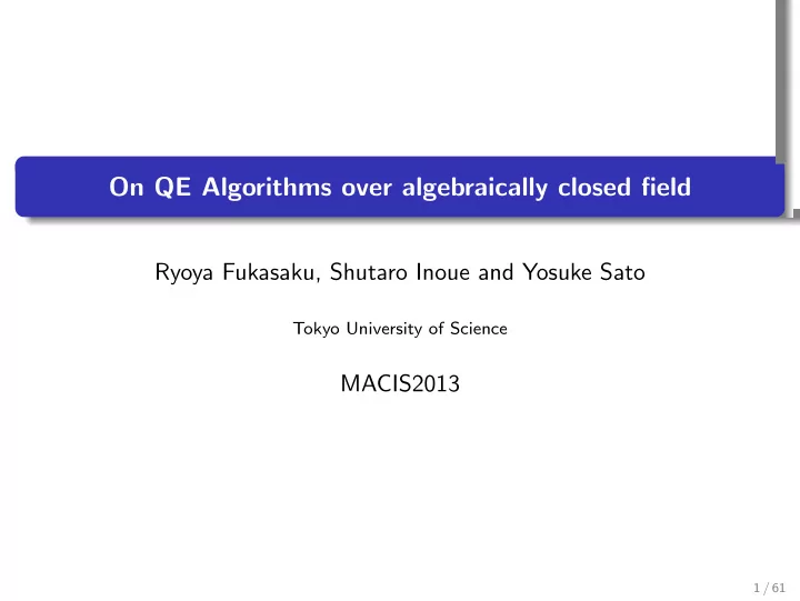
. On QE Algorithms over algebraically closed field . Ryoya Fukasaku, Shutaro Inoue and Yosuke Sato Tokyo University of Science MACIS2013 1 / 61

Contents of my talks . . Background 1 Outline Basic formulas Existing algorithms Merits of each existing algorithms Demerits of each existing algorithms . . Definitions and Lemma 2 Definitions Lemma . . GCD-QE and CGS-QE 3 GCD-QE algorithm CGS-QE algorithm . . Suzuki-Sato’s CGS original algorithm 4 . . Hybrid-QE 5 Algorithm Example Computation experiment . . Conclusions and Future works 6 2 / 61

. Background 1 Outline Basic formulas Existing algorithms Merits of each existing algorithms Demerits of each existing algorithms . . Definitions and Lemma 2 Definitions Lemma . . GCD-QE and CGS-QE 3 GCD-QE algorithm CGS-QE algorithm . . Suzuki-Sato’s CGS original algorithm 4 . . Hybrid-QE 5 Algorithm Example Computation experiment . . Conclusions and Future works 6 3 / 61

Outline What is Quantifier Elimination over algebraically closed field(ACF QE) ? ACF QE is computing the equivalent formula eliminating quantifier from a first-order formula over ACF. . Example . Input ∃ x ∈ C ( x − a 1 = 0 ∧ x − a 2 = 0 ∧ x − a 1 a 2 ̸ = 0) Output a 1 = a 2 ∧ − a 2 + a 2 2 ̸ = 0 . 4 / 61

Outline What is Quantifier Elimination over algebraically closed field(ACF QE) ? ACF QE is computing the equivalent formula eliminating quantifier from a first-order formula over ACF. . Example . Input ∃ x ∈ C ( x − a 1 = 0 ∧ x − a 2 = 0 ∧ x − a 1 a 2 ̸ = 0) Output a 1 = a 2 ∧ − a 2 + a 2 2 ̸ = 0 . 5 / 61

Basic formulas K : field, K : the algebraic closure of K , A : free variables A 1 , . . . , A n , X : quantified variables X 1 , . . . , X m , f 1 , . . . , f r , g 1 , . . . , g s ∈ K [ A, X ] . Basic formula . n ( f 1 = 0 ∧ . . . ∧ f r = 0 ∧ g 1 ̸ = 0 ∧ . . . ∧ g s ̸ = 0) ∃ X ∈ K . . Basic formula . n ( f 1 = 0 ∧ . . . ∧ f r = 0 ∧ g 1 . . . g s ̸ = 0) ∃ X ∈ K . The above formulas are equivalent. General ACF QE can return by QE the above basic formulas. 6 / 61

Basic formulas K : field, K : the algebraic closure of K , A : free variables A 1 , . . . , A n , X : quantified variables X 1 , . . . , X m , f 1 , . . . , f r , g 1 , . . . , g s ∈ K [ A, X ] . Basic formula . n ( f 1 = 0 ∧ . . . ∧ f r = 0 ∧ g 1 ̸ = 0 ∧ . . . ∧ g s ̸ = 0) ∃ X ∈ K . . Basic formula . n ( f 1 = 0 ∧ . . . ∧ f r = 0 ∧ g 1 . . . g s ̸ = 0) ∃ X ∈ K . The above formulas are equivalent. General ACF QE can return by QE the above basic formulas. 7 / 61

Existing algorithms The existing algorithms of ACF QE : . . 1 Method based on greatest common divisor (GCD-QE) . . 2 Method based on comprehensive Groebner system (CGS-QE) . . 3 Method based on characteristic sets and regular chains(CSRC-QE) The problems of the existing algorithms : Computation speed The computation speed of GCD-QE and CGS-QE is slow. Representation of output result The representation of output result of GCD-QE and CSRC-QE is generally complicated. 8 / 61

Existing algorithms The existing algorithms of ACF QE : . . 1 Method based on greatest common divisor (GCD-QE) . . 2 Method based on comprehensive Groebner system (CGS-QE) . . 3 Method based on characteristic sets and regular chains(CSRC-QE) The problems of the existing algorithms : Computation speed The computation speed of GCD-QE and CGS-QE is slow. Representation of output result The representation of output result of GCD-QE and CSRC-QE is generally complicated. 9 / 61

Merits of each existing algorithms GCD-QE The computation of ACF QE for one segment is often fast. CGS-QE By recent research we can compute a CGS with almost a minimum number of segments, which give us a very simple QE formula. CSRC-QE The computation of ACF QE is often fast. 10 / 61

Demerits of each existing algorithms GCD-QE We generally have a huge number of segments which makes the QE formula complicated, further we also need long computation time. CGS-QE We have to use new variables for inequations, which sometimes makes computation very heavy. CSRC-QE The representation of output result is generally complicated. 11 / 61

Demerits of each existing algorithms . . Example . ∃ ( x, y, z ) ∈ C 3 axz + xy + yz = 0 ∧ axyz + axy + axz +1 = 0 ∧ axz − az + yz − x − y = 0 . Output of GCD-QE : a 2 − 3 a + 3 = 0 ∨ a ̸ = 0 ∨ (16 a 8 − 144 a 7 + 504 a 6 − 864 a 5 + 729 a 4 − 135 a 3 − 324 a 2 + 405 a − 81 = 0 ∧ − a 2 + 3 a − 3 ̸ = 0) Output of CGS-QE : a ̸ = 0 Output of CSRC-QE : a ( a + 1)( a 2 − 3 a + 3) ̸ = 0 ∨ a 2 − 3 a + 3 = 0 ∨ a + 1 = 0 The output of CGS-QE is the most simple of 3 outputs. 12 / 61

Demerits of each existing algorithms . . Example . ∃ ( x, y, z ) ∈ C 3 axz + xy + yz = 0 ∧ axyz + axy + axz +1 = 0 ∧ axz − az + yz − x − y = 0 . Output of GCD-QE : a 2 − 3 a + 3 = 0 ∨ a ̸ = 0 ∨ (16 a 8 − 144 a 7 + 504 a 6 − 864 a 5 + 729 a 4 − 135 a 3 − 324 a 2 + 405 a − 81 = 0 ∧ − a 2 + 3 a − 3 ̸ = 0) Output of CGS-QE : a ̸ = 0 Output of CSRC-QE : a ( a + 1)( a 2 − 3 a + 3) ̸ = 0 ∨ a 2 − 3 a + 3 = 0 ∨ a + 1 = 0 The output of CGS-QE is the most simple of 3 outputs. 13 / 61

Today Main Theme Today we introduce Hybrid-QE for the following point. Return fast. Return simple output. 14 / 61

. Background 1 Outline Basic formulas Existing algorithms Merits of each existing algorithms Demerits of each existing algorithms . . Definitions and Lemma 2 Definitions Lemma . . GCD-QE and CGS-QE 3 GCD-QE algorithm CGS-QE algorithm . . Suzuki-Sato’s CGS original algorithm 4 . . Hybrid-QE 5 Algorithm Example Computation experiment . . Conclusions and Future works 6 15 / 61

Definitions m m ∈ N , S 1 , . . . , S t ⊆ K . Definition . m . { S 1 , . . . , S t } is a partition of K m ) : ⇔ ( ∀ i, j ( i ̸ = j ⇒ S i ∩ S j = ∅ )) ∧ ( S 1 ∪ . . . ∪ S t = K . We call each S i segment. S i is represented by a set which subtracts a variety from a variety. We identify S i with its defining formula. m F, G 1 , . . . , G t : finite subsets of K [ A, X ] , { S 1 , . . . , S t } : a partition of K . Definition . { ( S 1 , G 1 ) , . . . , ( S t , G t ) } is a CGS of ⟨ F ⟩ . : ⇔ ∀ a ∈ S i G i ( a ) is a Groebner basis(GB) of ⟨ F ( a ) ⟩ for each i , where F ( a ) = { f ( a, X ) : f ∈ F } ⊂ K [ X ] . . 16 / 61

Definitions m m ∈ N , S 1 , . . . , S t ⊆ K . Definition . m . { S 1 , . . . , S t } is a partition of K m ) : ⇔ ( ∀ i, j ( i ̸ = j ⇒ S i ∩ S j = ∅ )) ∧ ( S 1 ∪ . . . ∪ S t = K . We call each S i segment. S i is represented by a set which subtracts a variety from a variety. We identify S i with its defining formula. m F, G 1 , . . . , G t : finite subsets of K [ A, X ] , { S 1 , . . . , S t } : a partition of K . Definition . { ( S 1 , G 1 ) , . . . , ( S t , G t ) } is a CGS of ⟨ F ⟩ . : ⇔ ∀ a ∈ S i G i ( a ) is a Groebner basis(GB) of ⟨ F ( a ) ⟩ for each i , where F ( a ) = { f ( a, X ) : f ∈ F } ⊂ K [ X ] . . 17 / 61

Definitions m m ∈ N , S 1 , . . . , S t ⊆ K . Definition . m . { S 1 , . . . , S t } is a partition of K m ) : ⇔ ( ∀ i, j ( i ̸ = j ⇒ S i ∩ S j = ∅ )) ∧ ( S 1 ∪ . . . ∪ S t = K . We call each S i segment. S i is represented by a set which subtracts a variety from a variety. We identify S i with its defining formula. m F, G 1 , . . . , G t : finite subsets of K [ A, X ] , { S 1 , . . . , S t } : a partition of K . Definition . { ( S 1 , G 1 ) , . . . , ( S t , G t ) } is a CGS of ⟨ F ⟩ . : ⇔ ∀ a ∈ S i G i ( a ) is a Groebner basis(GB) of ⟨ F ( a ) ⟩ for each i , where F ( a ) = { f ( a, X ) : f ∈ F } ⊂ K [ X ] . . 18 / 61

Lemma f 1 , . . . , f r , g 1 , . . . , g s ∈ K [ A, X ] . Lemma . The following formulas is equivalent. n ( f 1 = 0 ∧ . . . ∧ f r = 0 ∧ g 1 ̸ = 0 ∧ . . . ∧ g s ̸ = 0) ∃ X ∈ K n ( g 1 . . . g s ∈ √ ¬ ( ∀ X ∈ K ⟨ f 1 , . . . , f r ⟩ )) s + n ( f 1 = 0 ∧ . . . ∧ f r = 0 ∧ 1 − Z 1 g 1 = 0 ∧ . . . ∧ 1 − Z s g s = 0) ∃ ( Z, X ) ∈ K . 19 / 61

. Background 1 Outline Basic formulas Existing algorithms Merits of each existing algorithms Demerits of each existing algorithms . . Definitions and Lemma 2 Definitions Lemma . . GCD-QE and CGS-QE 3 GCD-QE algorithm CGS-QE algorithm . . Suzuki-Sato’s CGS original algorithm 4 . . Hybrid-QE 5 Algorithm Example Computation experiment . . Conclusions and Future works 6 20 / 61

GCD-QE algorithm X : a quantified variable, f 1 , . . . , f r , g ∈ K [ A, X ] . Basic formula . ∃ X ∈ K ( f 1 = 0 ∧ . . . ∧ f r = 0 ∧ g ̸ = 0) . . . Compute parametric GCD’s s.t. 1 g i ( a, X ) := GCD ( f 1 ( a, X ) , . . . , f r ( a, X )) m for a ∈ S i , where { S 1 , . . . , S t } is a partition of K . . √ Refine each segment to S ′ i s.t. ¬ ( ∀ a ∈ S i ∀ X ∈ K ( g ∈ ⟨ g i ( a, X ) ⟩ )) ; 2 . . Return ∪ S ′ i ; 3 We can eliminate many quantified variables by recursive application. 21 / 61