On Cholesky structures on real symmetric matrices and their - PowerPoint PPT Presentation
On Cholesky structures on real symmetric matrices and their applications Hideyuki ISHI (Osaka City University) Virtual Conference Mathematical Methods of Modern Statistics 2, CIRM, June 2020. 1 Cholesky structure : a generalization of
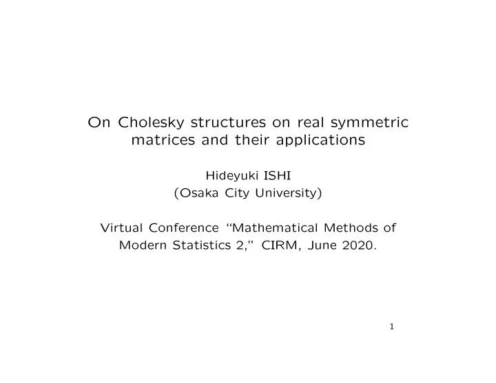
On Cholesky structures on real symmetric matrices and their applications Hideyuki ISHI (Osaka City University) Virtual Conference “Mathematical Methods of Modern Statistics 2,” CIRM, June 2020. 1
Cholesky structure : a generalization of Fill-in free property of a sparse matrix with respect to the Cholesky decomposition − → Exact calculation for Gaussian Selection model associ- ated to decomposable graph with symmetry of vertex permutation Plan: § 1. Cholesky structure § 2. Colored graphical model § 3. Gaussian selection model with a quasi-Cholesky structure Joint with P. Graczyk, B. Ko� lodziejek and H. Massam 2
§ 1. Cholesky structure. P n := { x ∈ Sym( n, R ) | x is positive definite } , { } h n := T = ( T ij ) ∈ Mat( n, R ) | T ij = 0 ( i < j ) , H n := { T ∈ h n | T ii > 0 ( i = 1 , . . . , n ) } . Fact. One has a bijection H n ∋ T �→ T t T ∈ P n . In other words, ∀ x ∈ P n ∃ 1 T x ∈ H n s.t. x = T x t T x (Cholesky decomposition) . When x is sparse, T x is sometimes sparse, too. x 11 x 21 0 0 x 21 x 22 x 32 0 For example, if x = ∈ P 4 , 0 x 32 x 33 x 43 0 0 x 43 x 44 0 0 0 T 11 0 0 T 21 T 22 then T x is of the form . 0 0 T 32 T 33 0 0 T 43 T 44 3
x 11 x 21 0 0 x 51 x 21 x 22 x 32 0 0 If x = 0 x 32 x 33 x 43 0 ∈ P 5 , then T x is 0 0 x 43 x 44 x 54 x 51 0 0 x 54 x 55 T 11 0 0 0 0 T 21 T 22 0 0 0 of the form 0 T 32 T 33 0 0 . 0 0 T 43 T 44 0 T 51 T 52 T 53 T 54 T 55 We have two fill-ins at T 52 and T 53 . 4
Let Z 1 be a vector subspace of Sym(5 , R ) consisting of x 11 x 21 0 0 x 51 x 21 x 22 x 32 0 0 x = 0 0 , and consider a subspace x 32 x 33 x 43 0 0 x 43 x 44 x 54 0 0 x 51 x 54 x 55 of h 5 spanned by T x with x ∈ Z 1 ∩P 5 . Then we see that dim span R { T x | x ∈ Z 1 ∩ P 5 } = dim Z 1 + 2 . On the other hand, if Z 2 ⊂ Sym(4 , R ) is the space of x 11 x 21 0 0 x 21 x 22 x 32 0 x = , then 0 x 32 x 33 x 43 0 0 x 43 x 44 dim span R { T x | x ∈ Z 2 ∩ P 4 } = dim Z 2 . 5
Definition 1. Let Z be a vector subspace of Sym( n, R ) such that I n ∈ Z . We say that Z has a Cholesky struc- ture if dim span { T x | x ∈ Z ∩ P n } = dim Z . 0 ( i < j ) , For x ∈ Sym( n, R ), define x ∨ ∈ h n by ( x ∨ ) ij := x ii / 2 ( i = j ) , x ij ( i > j ) , and ∧ ∨ + ∧ x := t ( x ∨ ). Then x = x x . Let Z ∨ denote the { } space x ∨ | x ∈ Z ⊂ h n . If I n ∈ Z , then Z ∨ equals the tangent space of { T x | x ∈ Z ∩ P n } ⊂ H n at I n , so that Z ∨ ⊂ span { T x | x ∈ Z ∩ P n } . 6
Theorem 2. Let Z be a vector subspace of Sym( n, R ) such that I n ∈ Z . Then the following are all equivalent: (i) Z has a Cholesky structure. (ii) span { T x | x ∈ Z ∩ P n } = Z ∨ . ∧ (iii) ∀ x ∈ Z x x ∈ Z . ∨ ∨ ∩ H n ∋ T �→ T t T ∈ Z ∩ P n . (iv) One has a bijection Z (i) ⇔ (ii) is obvious, (ii) ⇒ (iii) is easy, and (iv) ⇒ (ii) is trivial. A crucial part is (iii) ⇒ (iv). ∧ ∧ For x, y ∈ Sym( n, R ), define x ⋄ y := 2( x y + y x ) ∈ Sym( n, R ). ∨ ∨ Then x ⋄ I n = I n ⋄ x = x , and (iii) is equivalent to Z ⋄ Z ⊂ Z i.e. ∀ x, y ∈ Z x ⋄ y ∈ Z . Temporally, we say that Z ⊂ Sym( n, R ) is a Cholesky algebra if I n ∈ Z and Z ⋄ Z ⊂ Z . 7
Let Z ⊂ Sym( n, R ) be a Cholesky algebra and W ⊂ Mat( n, m, R ) a subspace such that u ∈ W ⇒ u t u ∈ Z . Then { ( ) } t u cI m E ( Z ; W ) := | c ∈ R , u ∈ W , x ∈ Z u x ⊂ Sym( m + n, R ) is a Cholesky algebra because ( c 2 / 4) I m c t u/ 2 ( ( c/ 2) I m ) ( ( c/ 2) I m t u ) 0 ∈ E ( Z , W ) . = ∧ ∧ u x x + u t u cu/ 2 x 0 x ∨ ∨ Starting from one-dimensional algebra R I n ⊂ Sym( n, R ), we obtain Cholesky algebras by repetition of this exten- sion procedure. 8
For example, let Z be the set of symmetric matrices of the form 0 0 c 1 a 0 0 c 1 a 0 a c 2 b 0 a b c 3 Setting W 1 := R I 2 and W 2 := R , we have Z = E ( E ( R ; W 2 ); W 1 ). We say that a Cholesky algebra Z is standard if Z = R I n or Z = E ( E ( · · · ( E ( R I s ; W r − 1 ); · · · ); W 2 ); W 1 ) with appropriate vector spaces W 1 , W 2 , . . . , W r − 1 . 9
Theorem 3. Any Cholesky algebra is isomorphic to a standard one, and the isomorphism is given by an ap- propriate permutation of rows and columns. For example, the Cholesky algebra Z of matrices a b 0 0 b c 0 0 0 0 a b 0 0 b d is isomorphic to the Cholesky algebra Z ′ of matrices 0 0 1 0 0 0 0 0 1 0 0 0 a b a b 0 0 0 0 1 0 0 0 0 0 1 0 a b b c = 0 0 0 1 0 0 0 0 0 1 0 0 b c a b 0 b 0 d 0 0 0 1 0 0 b d 0 0 0 1 ( ) 1 2 3 4 by the permutation (23) = . 1 3 2 4 10
The crucial part of Theorem 2 (i.e. (iii) ⇒ (iv)) fol- lows from Theorem 3. Eventually, we conclude that Z has a Cholesky structure if and only if Z is a Cholesky algebra. Definition 4. We say that a subspace Z of Sym( n, R ) has a quasi-Cholesky structure if there exists an invert- ible matrix A ∈ GL ( n, R ) such that Z A := { } Ax t A | x ∈ Z has a Cholesky structure. For example, a vector space Z ⊂ Sym(4 , R ) consisting a b 0 0 b c d 0 of x = , corresponding to a colored graph 0 d c b 0 0 b a b d b − a , has a quasi-Cholesky structure. a − c − c 11
1 0 0 − 1 1 0 0 1 1 Indeed, putting A := , we have √ 0 1 − 1 0 2 0 1 1 0 a b 0 0 a 0 b 0 b c d 0 0 a 0 b t A = A , 0 d c b b 0 c − d 0 0 0 b a 0 b 0 c + d so that 0 0 a b 0 a 0 b Z A = | a, b, c, d ∈ R , b 0 c 0 0 b 0 d which has a Cholesky structure. 12
§ 2. Colored graphical model Let G = ( V, E ) be an undirected graph with V = { 1 , · · · , n } and E ⊂ V × V . The graph G is said to be decomposable or chordal if any cycle in G of length ≥ 4 has a chord. Let Z G ⊂ Sym( n, R ) be the space of x = ( x ij ) for which x ij = 0 if i � = j and ( i, j ) �∈ E . It is known that, if G is decomposable and V is labeled appropriately, then each x ∈ Z G is decomposed as x = T x t T x without fill-ins. In our terminology, Z G has a Cholesky structure. For example, when G = 1 − 2 − 3 − 4, then Z G is the 0 0 x 11 x 21 0 x 21 x 22 x 32 vector space of x = . 0 x 32 x 33 x 43 0 0 x 43 x 44 13
Let Aut( G ) be the set of permutations σ ∈ S n such that ( σ ( i ) , σ ( j )) ∈ E ⇔ ( i, j ) ∈ E . Let Γ be a subgroup of Aut( G ), and define Z Γ { } G := x ∈ Z G | ∀ σ ∈ Γ ∀ i, j ∈ V x σ ( i ) σ ( j ) = x ij , which corresponds to the graph G whose vertices and edges are colored so that the objects mapped each other by Γ have the same color. For example, if G = 1 − 2 − 3 − 4 with Γ = Aut( G ) = { id, (14)(23) } . Then we have a colored graph 1 − 2 − 3 − 4 and a b 0 0 0 b c d Z Γ G = | a, b, c, d ∈ R . 0 d c b 0 0 b a 14
Let G be a decomposable and Γ any Theorem 4. subgroup of Aut( G ). Then Z Γ G ⊂ Sym( n, R ) has a quasi- Cholesky structure. A crucial point is how to find A ∈ GL ( n, R ) for which G ) A has a Cholesky structure. ( Z Γ Thanks to Theorem 4, we can generalize analysis on Z G by Letac-Massam (2007) to Z Γ G . 15
§ 3. Gaussian selection model with a quasi-Cholesky structure. Let Z be a vector subspace of Sym( n, R ) such that P Z = Z ∩ P n is non-empty. We consider a statistical N n (0 , Σ) | Σ − 1 ∈ P Z { } model M := , where N n (0 , Σ) stands for the multivariate zero-mean normal law with covariant matrix Σ. Let π Z : Sym( n, R ) → Z be the orthogonal projection with respect to the trace inner product. Let X 1 , X 2 , . . . , X s be i. i. d. obeying N n (0 , Σ) with Σ − 1 ∈ P Z . Then a Z - valued random matrix Y := π Z ( X 1 t X 1 + · · · + X s t X s ) / 2 is a sufficient statistics of the model M . Let W s, Σ de- note the law of Y , which we call the Wishart law for the model M . 16
Recommend
More recommend
Explore More Topics
Stay informed with curated content and fresh updates.
