On asymmetric quantum hypothesis testing JMP, Vol 57, 6, - PowerPoint PPT Presentation

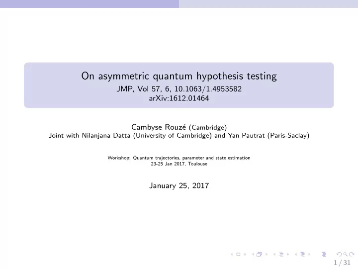
On asymmetric quantum hypothesis testing JMP, Vol 57, 6, 10.1063/1.4953582 arXiv:1612.01464 Cambyse Rouz´ e (Cambridge) Joint with Nilanjana Datta (University of Cambridge) and Yan Pautrat (Paris-Saclay) Workshop: Quantum trajectories, parameter and state estimation 23-25 Jan 2017, Toulouse January 25, 2017 1 / 31

Overview Motivation: the quantum Stein lemma and its refinements 1 Second-order asymptotics in Stein’s lemma 2 Some examples 3 Finite sample size quantum hypothesis testing: the i.i.d. case 4 2 / 31

Motivation: the quantum Stein lemma and its refinements Framework Let H finite dimensional Hilbert space, ρ, σ ∈ D ( H ) + , set of states on H Goal is to distinguish between: ρ (null hypothesis) and σ (alternative hypothesis) . A test is a POVM { T , 1 − T } , T ∈ B ( H ), 0 ≤ T ≤ 1 Errors when guessing are therefore given by: α ( T ) = Tr( ρ ( 1 − T )) type I error β ( T ) = Tr( σ T ) type II error Asymmetric case, minimize the type II error while controlling the type I error: β ( ǫ ) = 0 ≤ T ≤ 1 { β ( T ) | α ( T ) ≤ ǫ } . inf 3 / 31

Motivation: the quantum Stein lemma and its refinements Size-dependent hypothesis testing Let H n a sequence of Hilbert spaces, { ρ n } n ∈ N , { σ n } n ∈ N ∈ D ( H n ) + . Examples: the i.i.d. case: ρ n = ρ ⊗ n σ n = σ ⊗ n . vs . Gibbs states on a lattice Λ n of size | Λ n | = n d : − βρ H ρ − βσ H σ e Λ n e Λ n ρ n := vs . σ n := � . − βσ H σ − βρ H ρ � � � Tr e Λ n Tr e Λ n Quasi-free fermions on a lattice etc. Question: Given a uniform bound ǫ on the type I errors, how quickly does β n ( ǫ ) decrease with n ? 4 / 31

Motivation: the quantum Stein lemma and its refinements First-order asymptotics First proved in the i.i.d. setting Theorem (Quantum Stein’s lemma Hiai&Petz91, Ogawa&Nagaoka00) When ρ n = ρ ⊗ n , and σ n = σ ⊗ n , − 1 n log β n ( ǫ ) → D ( ρ � σ ) , ∀ ǫ ∈ (0 , 1) , where D ( ρ � σ ) = Tr( ρ (log ρ − log σ )) Umegaki’s relative entropy. r < D ( ρ � σ ) ⇒ α − 1 n →∞ − 1 n log min { α ( T n ) : β ( T n ) ≤ e − nr } := lim sup [ r − D α ( ρ � σ )] , α 0 <α< 1 r > D ( ρ � σ ) ⇒ n →∞ − 1 α − 1 n log max { (1 − α ( T n )) : β ( T n ) ≤ e − nr } = sup [ r − D ∗ α ( ρ � σ )] , where lim α 1 <α 1 α − 1 log Tr( ρ α σ 1 − α ) D α ( ρ � σ ) : = R´ enyi- α divergence, 1 1 − α D ∗ α − 1 log Tr( ρ 1 / 2 σ α ρ 1 / 2 ) α α ( ρ � σ ) : = sandwiched R´ enyi- α divergence. 5 / 31

Motivation: the quantum Stein lemma and its refinements Interpretation of Stein’s lemma 1 α (1) ∞ 0 t 1 D ( ρ || σ ) 1 α (1) ∞ = 0 ≤ T n ≤ 1 { lim sup inf α ( T n ) : − lim inf n log β ( T n ) ≥ t 1 } . n n Discontinuity of α (1) ∞ : manifestation of coarse-grained analysis. Question: can we better quantify the behaviour of the asymptotic type I error by adding a sub-exponential term for the type II error? 1 1 Lots of generalisations to the non i.i.d. framework: Bjelakovic&Siegmund-Schultze04, Bjelakovic,&Deuschel&Krueger&Seiler&Siegmund-Schultze&Szkola08, Hiai&Mosonyi&Ogawa08, Mosonyi&Hiai&Ogawa&Fannes08, Brandao&Plenio10, Jaksic&Ogata&Pillet&Seiringer12, etc. 6 / 31

Second-order asymptotics in Stein’s lemma Motivation: the quantum Stein lemma and its refinements 1 Second-order asymptotics in Stein’s lemma 2 Some examples 3 Finite sample size quantum hypothesis testing: the i.i.d. case 4 7 / 31

Second-order asymptotics in Stein’s lemma Second-order asymptotics in the i.i.d. case Tomamichel&Hayashi13 and Li14 proved the following second-order result: Theorem (Second-order asymptotics: the i.i.d. case Tomamichel&Hayashi13, Li14 ) When ρ n = ρ ⊗ n and σ n = σ ⊗ n , − log β n ( ǫ ) = nD ( ρ � σ ) + √ ns 1 ( ǫ ) + O (log n ) , � V ( ρ � σ )Φ − 1 ( ǫ ) , s 1 ( ǫ ) := where V ( ρ � σ ) = Tr( ρ (log ρ − log σ ) 2 ) − D ( ρ � σ ) 2 quantum information variance , and Φ the cumulative distribution function of law N (0 , 1) . 1 α (2) ∞ 1 2 t 2 0 1 � α (2) � � � � ∞ ( t 2 ) = inf lim sup α ( T n ) | − lim inf log β n ( T n )+ n D ( ρ || σ ) ≥ t 2 = Φ( t 2 / V ( ρ � σ )) . √ n n 0 ≤ Tn ≤ 1 n 8 / 31

Second-order asymptotics in Stein’s lemma Main result 1: Second-order asymptotics in the non-i.i.d. scenario For a given strictly increasing sequence of weights w n , under some conditions (see later), the quantum information variance rate 1 v ( { ρ n } , { σ n } ) = lim V ( ρ n � σ n ) n →∞ w n is well-defined, and: Theorem (DPR16) Fix ǫ ∈ (0 , 1) . Define t ∗ � v ( { ρ n } , { σ n } ) Φ − 1 ( ǫ ) . 2 ( ǫ ) = Then + ∞ o ( √ x ) such that ∀ n ∈ N and any Optimality: ∀ t 2 > t ∗ 2 ( ǫ ) there exists a function f t 2 ( x ) = sequence of tests T n : − log β ( T n ) ≤ D ( ρ n || σ n ) + √ w n t 2 + f t 2 ( w n ) , (1) + ∞ o ( √ x ) , there exists a sequence of test T n such that Achievability: ∀ t 2 < t ∗ 2 ( ǫ ) , ∀ f ( x ) = for n large enough: − log β n ( T n ) ≥ D ( ρ n || σ n ) + √ w n t 2 + f ( w n ) . (2) The i.i.d. case of Tomamichel&Hayashi13 and Li14 follows (Bryc ← CLT). The Berry-Esseen theorem even provides information on third order: � nV ( ρ � σ )Φ − 1 ( ǫ ) + O (log n ) , − log β n ( ǫ ) = nD ( ρ � σ ) + 9 / 31

Second-order asymptotics in Stein’s lemma Key tools 1: the relative modular operator The relative modular operator is a generalisation of the Radon-Nikodym derivative for general von Neuman algebras. In finite dimensions, for two faithful states, it reduces to: A �→ ρ A σ − 1 . ∆ ρ | σ : B ( H ) → B ( H ) , ∆ ρ | σ is a positive operator, admits a spectral decomposition. Quantities of relevance can be rewritten in terms of ∆ ρ | σ : D ( ρ � σ ) = � ρ 1 / 2 , log(∆ ρ | σ )( ρ 1 / 2 ) � , where � A , B � = Tr( A ∗ B ) . Ψ s ( ρ | σ ) := log Tr( ρ 1+ s σ − s ) = log � ρ 1 / 2 , ∆ s ρ | σ ( ρ 1 / 2 ) � Define X to be the classical random variable taking values on spec(log ∆ ρ | σ ) such that for any measurable f : spec(log ∆ ρ | σ ) → R , � ρ 1 / 2 , f (log ∆ ρ | σ )( ρ 1 / 2 ) � ≡ E [ f ( X )] . f : x �→ x ⇒ E [ X ] = D ( ρ � σ ), f : x �→ e sx ⇒ log E [e sX ] = log � ρ 1 / 2 , e s log ∆ ρ | σ ( ρ 1 / 2 ) � ≡ Ψ s ( ρ | σ ), the cumulant-generating function. 10 / 31

Second-order asymptotics in Stein’s lemma Key tools 2: Bryc’s theorem The following theorem is a non i.i.d. generalization of the Central limit theorem: Theorem (Bryc’s theorem Bryc93) Let ( X n ) n ∈ N be a sequence of random variables, and ( w n ) n ∈ N an increasing sequence of weights. If there exists r > 0 such that: � � e zXn ∀ n ∈ N , H n ( z ) := log E is analytic in the complex open ball B C (0 , r ) , 1 H ( x ) = lim n →∞ wn H n ( x ) exists ∀ x ∈ ( − r , r ) , 1 sup n ∈ N sup z ∈ B C (0 , r ) wn | H n ( z ) | < + ∞ , then H is analytic on B C (0 , r ) and X n − H ′ n (0) d 0 , H ′′ (0) � � √ w n − → n →∞ N , 11 / 31

Second-order asymptotics in Stein’s lemma The working condition Take X n associated to log ∆ ρ n | σ n , ρ 1 / 2 ⇒ H n ( z ) = Ψ z ( ρ n | σ n ). n The conditions of Bryc’s theorem translate into: Condition Let { w n } an increasing sequence of weights. Assume there exists r > 0 such that ∀ n ∈ N , z → Ψ z ( ρ n | σ n ) is analytic in the complex open ball B C (0 , r ) , 1 H ( x ) = lim n →∞ wn Ψ z ( ρ n | σ n ) exists ∀ x ∈ ( − r , r ) , 1 sup n ∈ N sup z ∈ B C (0 , r ) wn | Ψ z ( ρ n | σ n ) | < + ∞ , Here H ′ n (0) = D ( ρ n � σ n ), By Bryc’s theorem, the quantum information variance rate 1 V ( ρ n � σ n ) ≡ H ′′ (0) v ( { ρ n } , { σ n } ) = lim w n n →∞ is well-defined. 12 / 31

Second-order asymptotics in Stein’s lemma Proof of achievability (2) We will need the following crucial technical lemma: Lemma (Li14, DPR16) Let ρ, σ ∈ D + ( H ) . For all L > 0 there exists a test T such that Tr( ρ ( 1 − T )) ≤ � ρ 1 / 2 , P (0 , L ) (∆ ρ | σ )( ρ 1 / 2 ) � Tr( σ T ) ≤ L − 1 . and (3) Let L n := exp( D ( ρ n � σ n ) + √ w n t 2 + f ( w n )), f ( x ) = ◦ ( √ x ). − log β ( T n ) ≥ D ( ρ n || σ n ) + √ w n t 2 + f ( w n ) (3) ⇒ ρ n 1 / 2 , P (0 , L n ) (∆ ρ n | σ n ) ρ n 1 / 2 � α ( T n ) ≤ � , ρ n 1 / 2 , P ( −∞ , log L n ) (log ∆ ρ n | σ n ) ρ n 1 / 2 � � = . � X n − D ( ρ n || σ n ) ≤ t 2 + f ( w n ) � = P ( X n ≤ log L n ) = P . √ w n √ w n � Bryc’s theorem ⇒ RHS converges to Φ( t 2 / v ( { ρ n } , { σ n } )) < ε ⇒ for n large enough, α ( T n ) ≤ ε. Optimality (1) follows similarly from a lower bound on the total error provided by Jaksic&Ogata&Pillet&Seiringer12. 13 / 31

Some examples Motivation: the quantum Stein lemma and its refinements 1 Second-order asymptotics in Stein’s lemma 2 Some examples 3 Finite sample size quantum hypothesis testing: the i.i.d. case 4 14 / 31

Some examples Quantum spin systems Lattice Z d . System prepared at each site: ∀ x , H x = H . Example: particle (spin ± 1 2 ): H x = C 2 . 15 / 31