OBSERVATIONAL COSMOLOGY Exercise 3 & 4 28.4.10 & 5.5.10 - PDF document

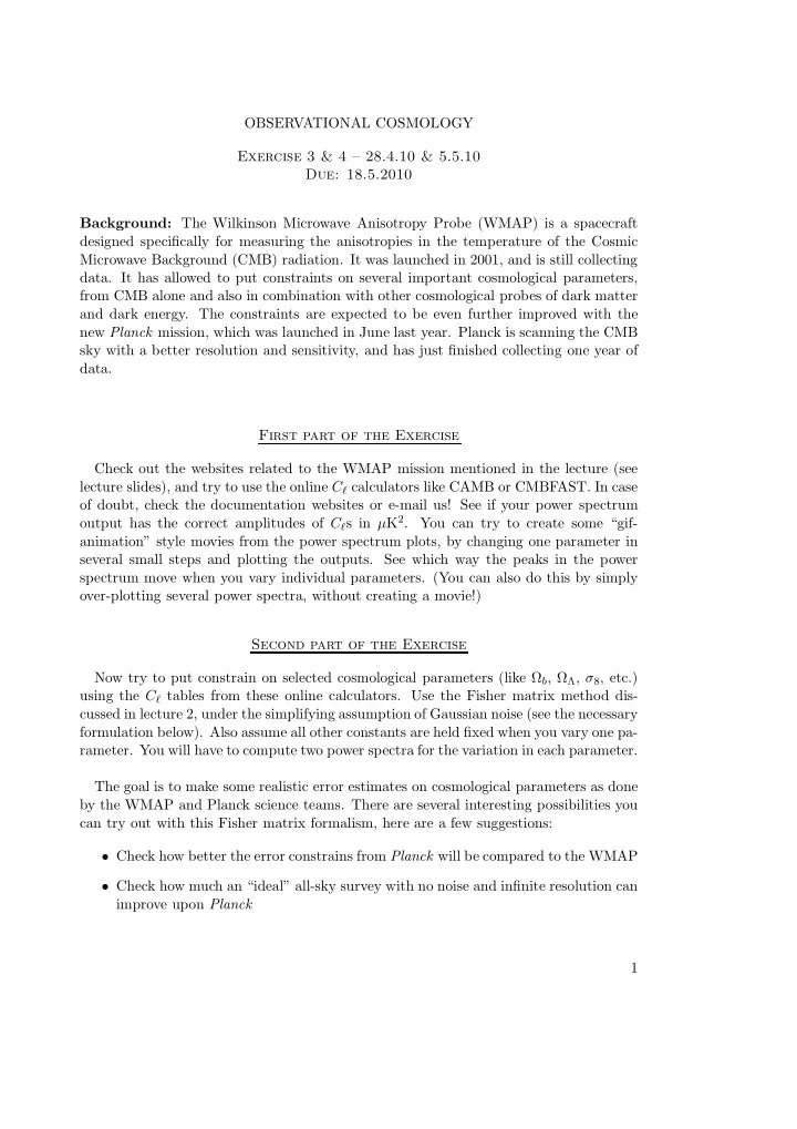
OBSERVATIONAL COSMOLOGY Exercise 3 & 4 – 28.4.10 & 5.5.10 Due: 18.5.2010 Background: The Wilkinson Microwave Anisotropy Probe (WMAP) is a spacecraft designed specifically for measuring the anisotropies in the temperature of the Cosmic Microwave Background (CMB) radiation. It was launched in 2001, and is still collecting data. It has allowed to put constraints on several important cosmological parameters, from CMB alone and also in combination with other cosmological probes of dark matter and dark energy. The constraints are expected to be even further improved with the new Planck mission, which was launched in June last year. Planck is scanning the CMB sky with a better resolution and sensitivity, and has just finished collecting one year of data. First part of the Exercise Check out the websites related to the WMAP mission mentioned in the lecture (see lecture slides), and try to use the online C ℓ calculators like CAMB or CMBFAST. In case of doubt, check the documentation websites or e-mail us! See if your power spectrum output has the correct amplitudes of C ℓ s in µ K 2 . You can try to create some “gif- animation” style movies from the power spectrum plots, by changing one parameter in several small steps and plotting the outputs. See which way the peaks in the power spectrum move when you vary individual parameters. (You can also do this by simply over-plotting several power spectra, without creating a movie!) Second part of the Exercise Now try to put constrain on selected cosmological parameters (like Ω b , Ω Λ , σ 8 , etc.) using the C ℓ tables from these online calculators. Use the Fisher matrix method dis- cussed in lecture 2, under the simplifying assumption of Gaussian noise (see the necessary formulation below). Also assume all other constants are held fixed when you vary one pa- rameter. You will have to compute two power spectra for the variation in each parameter. The goal is to make some realistic error estimates on cosmological parameters as done by the WMAP and Planck science teams. There are several interesting possibilities you can try out with this Fisher matrix formalism, here are a few suggestions: • Check how better the error constrains from Planck will be compared to the WMAP • Check how much an “ideal” all-sky survey with no noise and infinite resolution can improve upon Planck 1

• Check what is the ℓ -range necessary for constraining your parameters: do you need to compute the power spectrum up to ℓ = 2000? • Check if COBE could constrain any of your parameters, with only measuring the power in the Sachs-Wolfe plateau (limits your C ℓ s to ℓ = 50) • (Make some of your own!) Method The Fisher matrix for the CMB is given by: ℓ max � − 2 ∂C ℓ (2 ℓ + 1) f sky ∂C ℓ � N e ℓ ( ℓ +1) σ 2 � C ℓ + Ω beam σ 2 F ij = , b 2 ∂s i ∂s j ℓ =2 where • ℓ is the multipole moment; • C ℓ is the angular power spectrum; • s i , s j are the two parameters you want to vary; • σ N is the noise per pixel (in µ K); • Ω beam = 1 . 13(FWHM) 2 is the solid angle subtended by each pixel (FWHM is the full width at half maximum of the beam, assuming it’s Gaussian); � • σ b = FWHM / 8 ln(2) is the width Gaussian beam; and • f sky is the fractional sky coverage (assume f sky = 0 . 8 for both WMAP and Planck) Here is a table with the WMAP and Planck survey capabilities, assuming one year of observation. Mission Frequency (GHz) σ N ( µK ) beam FWHM (arcmin) WMAP 94 49 13 Planck 143 6 . 0 7 . 1 Using the online tool of CAMB or CMBFAST to obtain the C ℓ ’s, 1. plot the two contributions to the covariance matrix of the CMB, the cosmic vari- ance and the noise per beam, versus the ℓ ’s; 2. plot the joint probability contours at 68 . 3% confidence level for a couple of cosmo- logical parameter (e.g. Ω b − Ω Λ ) and compare the WMAP result with the forecast for Planck (and try some other suggestions mentioned above). 2

Hints : � 2 � = ℓ ( ℓ +1) ∆ T • From CMBFAST one actually gets the dimensionless C ℓ , where T 0 2 π T 0 = 2 . 726 K. So you need to multiply the outputs with right factors to get C ℓ ’s in µK 2 ; • the FWHM has to be expressed in radians; • since you do not have an analytical expression for the C ℓ ’s as a function of the parameters, to make the derivatives for the Fisher matrix you have to generate different spectra with different values of the parameters and approximate ∂C ℓ s ≈ C ℓ (¯ s + ∆ s ) − C ℓ (¯ s − ∆ s ) | ¯ . ∂s i 2∆ s • The inverse of Fisher matrix is the noise covariance matrix � σ 2 � σ xy [ F ] − 1 = [ C ] = x (0.1) σ 2 σ xy y • The parameters of the error ellipse are calculated as follows: � a 2 = σ 2 x + σ 2 ( σ 2 x − σ 2 y ) 2 y + σ 2 + (0.2) xy 2 4 � b 2 = σ 2 x + σ 2 ( σ 2 x − σ 2 y ) 2 y + σ 2 − (0.3) xy 2 4 2 σ xy tan 2 θ = (0.4) σ 2 x − σ 2 y 3