Numerical tensor methods and their applications I.V. Oseledets 7 - PowerPoint PPT Presentation
Numerical tensor methods and their applications I.V. Oseledets 7 May 2013 I.V. Oseledets Numerical tensor methods and their applications All lectures 4 lectures, 2 May, 08:00 - 10:00: Introduction: ideas, matrix results, history. 7 May,
Numerical tensor methods and their applications I.V. Oseledets 7 May 2013 I.V. Oseledets Numerical tensor methods and their applications
All lectures 4 lectures, 2 May, 08:00 - 10:00: Introduction: ideas, matrix results, history. 7 May, 08:00 - 10:00: Novel tensor formats (TT, HT, QTT). 8 May, 08:00 - 10:00: Advanced tensor methods (eigenproblems, linear systems). 14 May, 08:00 - 10:00: Advanced topics, recent results and open problems. I.V. Oseledets Numerical tensor methods and their applications
Brief recap of Lecture 1 Previous lecture: I.V. Oseledets Numerical tensor methods and their applications
Brief recap of Lecture 1 Previous lecture: SVD and skeleton decompositions I.V. Oseledets Numerical tensor methods and their applications
Brief recap of Lecture 1 Previous lecture: SVD and skeleton decompositions A tensor is a d -way array: A ( i 1 , . . . , i d ) I.V. Oseledets Numerical tensor methods and their applications
Brief recap of Lecture 1 Previous lecture: SVD and skeleton decompositions A tensor is a d -way array: A ( i 1 , . . . , i d ) Key idea: separation of variables I.V. Oseledets Numerical tensor methods and their applications
Two classical formats Two classical formats: The canonical format The Tucker format I.V. Oseledets Numerical tensor methods and their applications
The canonical format Canonical format A ( i 1 , . . . , i d ) = � r α = 1 U 1 ( i 1 , α ) . . . U d ( i d , α ) dnr parameters (low!) No robust algorithms Uniqueness, important as a data model I.V. Oseledets Numerical tensor methods and their applications
Tucker format Tucker format A ( i 1 , . . . , i d ) = � α 1 ,...,α d G ( α 1 , . . . , α d ) U 1 ( i 1 , α 1 ) . . . U d ( i d , α d ) dnr + r d parameters (high!) SVD-based algorithms No uniqueness I.V. Oseledets Numerical tensor methods and their applications
Main question Can we find something inbetween? (Tucker and canonical) The tensor format that has: No curse of dimensionality SVD-based algorithms I.V. Oseledets Numerical tensor methods and their applications
Plan of lecture 2 History of novel formats The Tree-Tucker, Tensor Train, Hierarchical Tucker formats Their difference Concept of Tensor Networks Stability and quasioptimality Basic arithmetic (with illustration) Cross approximation formula (with illustrations) QTT-format (part 1) I.V. Oseledets Numerical tensor methods and their applications
History(0) In 2000-s there was a lot of work done on the canonical/Tucker formats in multilinear algebra: Beylkin и Mohlenkamp (2002), first to use as a format Hackbusch, Khoromskij, Tyrtyshnikov, Grasedyck I.V. Oseledets Numerical tensor methods and their applications
History Beginning of 2009, two papers: I. V. Oseledets, E. E. Tyrtyshnikov, Breaking the curse of dimensionality, or how to use SVD in many dimensions W. Hackbusch, S. K¨ uhn, A new scheme for the tensor representation Two hierarchical schemes: TT (TT=Tree Tucker) и HT(Hierarchical Tucker) I.V. Oseledets Numerical tensor methods and their applications
History It was almost immediately found, that Tree-Tucker can be rewritten in a much simpler algebraic way, called Tensor-Train. I.V. Oseledets Numerical tensor methods and their applications
History In March-April 2009 all the basic arithmetics was obtained for the TT-formats, with similar algorithms obtained for HT by different groups later on, but: HT are typically more complex There is no explicit advantage in practice I.V. Oseledets Numerical tensor methods and their applications
History June 2009 года: L. Grasedyck, Hierarchical singular value decomposition of tensors June 2009 года: O., Tyrtyshnikov, TT-cross approximation of multidimensional arrays - first skeleton decomposition formula in many dimensions. I.V. Oseledets Numerical tensor methods and their applications
History 2010, R. Schneider found that similar things were used in solid state physics (Matrix Product States), as a representation of certain states (but not as a mathematical instruments) White (1993), Ostlund и Rommer (1995), Vidal (2003). Approaches MCTDH/ML-MCTDH in quantum chemistry can be interperted as a HT-format. New mathematical tensor-based framework has emerged I.V. Oseledets Numerical tensor methods and their applications
History The topic is very “hot” and is full of new challenges. Merging of linear algebra and many different areas Old and new applications Numerical experiments are far ahead of the theoretical results Limitations? I.V. Oseledets Numerical tensor methods and their applications
Tensors and matrices Idea: if for matrices everything is good, let us transform tensors into matrices! I.V. Oseledets Numerical tensor methods and their applications
Tensors and matrices By reshaping! ( i 1 , . . . , i d ) = ( I , J ) , I = ( i 1 , i 4 ) , J = ( i 2 , i 3 , i 5 ) . A → B ( I , J ) - a matrix I.V. Oseledets Numerical tensor methods and their applications
First lemma Lemma 1 If A has canonical rank r then for any splitting B = A ( I , J ) rank B ≤ r I.V. Oseledets Numerical tensor methods and their applications
Second lemma B = UV ⊤ , still exponentially many parameters! Lemma 2 Let B = UV ⊤ with full-rank U and V Then, U = U ( I , α ) , V = V ( J , α ) can be considered as d 1 + 1 and d 2 + 1 tensors; then these tensors have canonical rank- r representations! I.V. Oseledets Numerical tensor methods and their applications
Dimension tree The process can be then applied recursively: We had a 9 dimensional tensor of canonical rank r , splitted into 4 and 5 indices, then replaced it by 5 = 4 + 1 and 6 = 5 + 1 dimensional tensors of canonical rank r . We can go on . . . I.V. Oseledets Numerical tensor methods and their applications
Dimension tree I.V. Oseledets Numerical tensor methods and their applications
Dimension tree Theorem: The number of leafs (3-d tensors) is exactly ( d − 2 ) Complexity is O ( dnr ) + ( d − 2 ) r 3 . I.V. Oseledets Numerical tensor methods and their applications
Equivalence to the tensor train(1) We quickly realized, that the tree is in fact not needed , and up to the permutation of the dimensions, Tensor train A ( i 1 , . . . , i d ) = � α 1 ,...,α d − 1 G 1 ( i 1 , α 1 ) G 2 ( α 1 , i 2 , α 2 ) . . . G d ( α d − 1 , i d ) I.V. Oseledets Numerical tensor methods and their applications
Tensor train (2) Tensor train A ( i 1 , . . . , i d ) = � α 1 ,...,α d − 1 G 1 ( i 1 , α 1 ) G 2 ( α 1 , i 2 , α 2 ) . . . G d ( α d − 1 , i d ) α 1 α 2 α 3 i 1 α 1 α 1 i 2 α 2 α 2 i 3 α 3 α 3 i 4 I.V. Oseledets Numerical tensor methods and their applications
Tensor train (3) Tensor train A ( i 1 , . . . , i d ) = G 1 ( i 1 ) G 2 ( i 2 ) . . . G d ( i d ) . α 1 α 2 α 3 α 4 i 1 i 2 i 3 i 4 i 5 The matrices G k ( i k ) have sizes r k − 1 × r k , r 0 = r d = 1, the numbers r k are called TT-ranks. I.V. Oseledets Numerical tensor methods and their applications
HT format The Hierachical Tucker format can be treated as sequential application of the Tucker decomposition: Compute the Tucker of an n × n × n × n × n array, get the core r × r × r × r × r Select pairs, reshape into a r 2 × r 2 × r 2 × r array Compute the Tucker decomposition (again), the factors will be r leaf r leaf r father - the same 3d-tensors Do it recursively The process is described by a binary tree I.V. Oseledets Numerical tensor methods and their applications
Tensor network concept All these formats can be interpreted as tensor networks: Canonical format Tucker format Linear Tensor Network (LTN) - TT-format Tree Tensor Network - HT/format What about more complex networks? I.V. Oseledets Numerical tensor methods and their applications
Tensor network concept (2) Multidimensional grids (PEPS-states) They are not closed! J. M. Landsburg, Y. Qi, K. Ye, On the geometry of tensor network states, arxiv.org/pdf/1105.4449.pdf The multidimensional states can be useful, but we will face all the hazards of the canonical format (again)! I.V. Oseledets Numerical tensor methods and their applications
Definition The tensor is said to be in the TT-format, if A ( i 1 , . . . , i d ) = G 1 ( i 1 ) G 2 ( i 2 ) . . . G d ( i d ) , where G k ( i k ) is a r k − 1 × r k matrix, r 0 = r d = 1 r k are called TT-ranks G k ( i k ) (which are in fact r k − 1 × n k × r k ) are called cores I.V. Oseledets Numerical tensor methods and their applications
TT in a nutshell A has canonical rank r → r k ≤ r TT-ranks are matrix ranks, TT-SVD All basic arithmetic, linear in d , polynomial in r Fast TENSOR ROUNDING TT-cross method, exact interpolation formula Q(Quantics, Quantized)-TT decomposition — binarization (or tensorization) of vectors, matrices I.V. Oseledets Numerical tensor methods and their applications
TT-ranks are matrix ranks Define unfoldings: A k = A ( i 1 . . . i k ; i k + 1 . . . i d ) , n k × n d − k matrix I.V. Oseledets Numerical tensor methods and their applications
TT-ranks are matrix ranks Define unfoldings: A k = A ( i 1 . . . i k ; i k + 1 . . . i d ) , n k × n d − k matrix Theorem: there exists a TT-decomposition with TT-ranks r k = rank A k I.V. Oseledets Numerical tensor methods and their applications
Recommend
More recommend
Explore More Topics
Stay informed with curated content and fresh updates.


