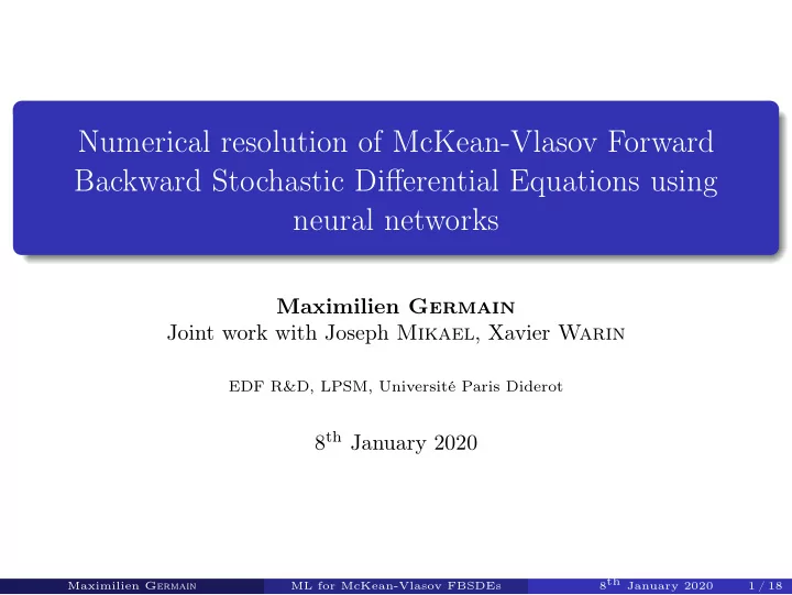
Numerical resolution of McKean-Vlasov Forward Backward Stochastic - PowerPoint PPT Presentation
Numerical resolution of McKean-Vlasov Forward Backward Stochastic Differential Equations using neural networks Maximilien Germain Joint work with Joseph Mikael , Xavier Warin EDF R&D, LPSM, Universit Paris Diderot 8 th January 2020 8th
Numerical resolution of McKean-Vlasov Forward Backward Stochastic Differential Equations using neural networks Maximilien Germain Joint work with Joseph Mikael , Xavier Warin EDF R&D, LPSM, Université Paris Diderot 8 th January 2020 8th January 2020 Maximilien Germain ML for McKean-Vlasov FBSDEs 1 / 18
McKean-Vlasov FBSDEs We solve general McKean-Vlasov FBSDEs of the form � t � t � X t = ξ + 0 b ( s, X s , Y s , Z s , L ( X s ) , L ( Y s ) , L ( Z s )) d s + 0 σ ( s, X s ) d W s � T � T Y t = g ( X T , L ( X T )) + t f ( s, X s , Y s , Z s , L ( X s ) , L ( Y s ) , L ( Z s ))d s − t Z s d W s with machine learning techniques. W s is a standard Brownian motion. The processes dynamics depend on their laws L ( · ) . In practise we restrict to cases when the law dependence only concerns probability moments. 8th January 2020 Maximilien Germain ML for McKean-Vlasov FBSDEs 2 / 18
Main motivation: Mean Field Games (MFG) Stochastic games introduced by (Lasry and Lions 2006), (Huang, Malhame, and Caines 2006) followed by (Carmona and Delarue 2012) dealing with a large number of interacting players. The empirical law of players states influences both the dynamics and cost. Applications Population dynamics (crowd, traffic jam, bird flocking...). Market interactions (Cardaliaguet and Lehalle 2019). Energy storage (Matoussi, Alasseur, and Ben Taher 2018), electric cars management. Social networks. 8th January 2020 Maximilien Germain ML for McKean-Vlasov FBSDEs 3 / 18
N players stochastic game Player i minimises a cost J i ( α 1 , · · · , α i , · · · , α N ) depending on the empirical distribution µ t = 1 � N k =1 δ X k t → mean field interaction. N �� T � f ( t, X i t , µ t , α i t ) d t + g ( X i min E T , µ T ) α i ∈ A 0 d X i t = b ( t, X i t , µ t , α i t ) d t + σ ( t, X i t , µ t ) d W i subject to t . Difficult problem in general. 8th January 2020 Maximilien Germain ML for McKean-Vlasov FBSDEs 4 / 18
Asymptotic control problem when N → + ∞ Given a family ( µ t ) t ∈ [0 ,T ] of probability measures we solve for a representative player �� T � f ( t, X µ t , µ t , α t ) d t + g ( X µ min E T , µ T ) α 0 d X µ t = b ( t, X µ t , µ t , α t ) d t + σ ( t, X µ subject to t , µ t ) d W t . Fixed point on probability measures µ t = L ( X µ t ) . Simpler than the N players game → unique player in the limit! Value function given by �� T � v µ ( t, x ) = inf f ( s, X s , µ s , α s ) d s + g ( X T , µ T ) | X t = x . α ∈A t E t 8th January 2020 Maximilien Germain ML for McKean-Vlasov FBSDEs 5 / 18
Optimality conditions HJB equation � ∂ t v + 1 2 Tr( σσ ⊤ ∂ 2 xx v ) + min α ∈A H ν t ( t, x, ∂ x v, α ) = 0 v ( T, x ) = g ( x, ν T ) coupled with Fokker-Planck equation: � ∂ t ν − 1 2 Tr( σσ ⊤ ∂ 2 α ν t ( t, x, ∂ x v )) ν ) = 0 xx ν ) − div( b ( t, x, ν t , ˆ ν (0 , · ) = ν 0 . Solved in (Achdou and Capuzzo-Dolcetta 2010) with finite differences methods. 8th January 2020 Maximilien Germain ML for McKean-Vlasov FBSDEs 6 / 18
Probabilistic point of view: McKean-Vlasov FBSDEs Y t = ∂ x v ( t, X t ) → stochastic Pontryagin principle α L ( X t ) ( t, X t , Y t )) d t + σ d W t d X t = b ( t, X t , L ( X t ) , ˆ X 0 = ξ = − ∂ x H L ( X t ) ( t, X t , Y t , ˆ α L ( X t ) ( t, X t , Y t )) d t + Z t d W t d Y t Y T = ∂ x g ( X T , µ T ) . In the form � t � t � X t = ξ + 0 b ( s, X s , Y s , Z s , L ( X s ) , L ( Y s ) , L ( Z s )) d s + 0 σ ( s, X s ) d W s � T � T Y t = g ( X T , L ( X T )) + t f ( s, X s , Y s , Z s , L ( X s ) , L ( Y s ) , L ( Z s ))d s − t Z s d W s 8th January 2020 Maximilien Germain ML for McKean-Vlasov FBSDEs 7 / 18
Advantages of machine learning techniques Curse of dimensionnality with finite differences methods if the state dimension is high ( ≥ 3 or 4 ). − → Some machine learning schemes solve nonlinear PDE in high dimension (10, 50 or even 100): - Deep BSDE method of (Han, Jentzen, and E 2017) - Deep Galerkin method of (Sirignano and Spiliopoulos 2017) - Deep Backward Dynamic Programming of (Huré, Pham, and Warin 2020). − → Open source libraries such as Tensorflow or Pytorch. − → Efficient computation on GPU nodes. 8th January 2020 Maximilien Germain ML for McKean-Vlasov FBSDEs 8 / 18
A global method Based on the Deep BSDE method of (Han, Jentzen, and E 2017) � t � t � X t = ξ + 0 b ( s, X s , Y s , Z s , L ( X s ) , L ( Y s ) , L ( Z s )) d s + 0 σ ( s, X s ) d W s � T � T Y t = g ( X T , L ( X T )) + t f ( s, X s , Y s , Z s , L ( X s ) , L ( Y s ) , L ( Z s ))d s − t Z s d W s Discretization: � X t i +1 = X t i + b ( t i , X t i , Y t i , Z t i , µ t i ) ∆ t i + σ ( t i , X t i ) ∆ W t i = Y t i − f ( t i , X t i , Y t i , Z t i , µ t i ) ∆ t i + Z θ ( t i , X t i )∆ W t i . Y t i +1 Y 0 is a variable and Z t i is approached by a neural network Z θ ( t i , · ) which � ( Y T − g ( X T , µ T )) 2 � minimizes the loss function E . The forward backward system is transformed into a forward form and an optimization problem. Also studied in (Fouque and Zhang 2019), (Carmona and Laurière 2019) in dimension 1 and with less generality. 8th January 2020 Maximilien Germain ML for McKean-Vlasov FBSDEs 9 / 18
Fixed point on probability measures Estimation of state and value function moments: Direct : use of current particles empirical law N b = 1 E [ X t i ] ( k +1) ≃ µ ( k +1) � X j t i . (1) t i N b j =1 Dynamic : keep in memory previously computed moments and average them with current particle moments N m N b µ ( k ) t i + � N b j =1 X j E [ X t i ] ( k +1) ≃ t i . (2) N b + N m N b Expectation : estimate E [ X t ] by an additional neural network. E [ X t ] ≃ Ψ κ ( t ) . (3) � � 2 � λ � N t � We add to the loss a term E Ψ κ ( t i ) − X t i . i =0 8th January 2020 Maximilien Germain ML for McKean-Vlasov FBSDEs 10 / 18
A local approach Inspired by (Huré, Pham, and Warin 2020). Z and Y are approximated by neural networks ( Z i m ( · ) , Y i m ( · )) { i ∈ � 0 ,N − 1 � } . At θ i θ i iteration m we simulate X i with the previously computed parameters θ i m . The X i ’s dynamics being frozen with parameters θ i m : First Y N is set to the terminal condition g ( X N , µ N ) . Then, we solve successively the local backward problems for i from N − 1 to 0 2 � � Y i +1 � � − Y i ti, Xi, Y i , Zi ∆ t − Zi . min Xi +1 � Xi � + f � Xi � � Xi � , µti � Xi � ∆ Wti E θi θi θi θi θi +1 θi m m m m m m +1 8th January 2020 Maximilien Germain ML for McKean-Vlasov FBSDEs 11 / 18
A linear quadratic test case: price impact Large number of traders who want to sell a portfolio at the same time. Example from (Carmona and Delarue 2018). �� T � � c α 2 � α t � 2 + c X d t + c g 2 � X t � 2 − γX t · µ t � 2 � X T � 2 min E α ∈ A 0 . � t subject to X t = x 0 + α s d s + σ W t 0 and the fixed point E [ α t ] = µ t . Optimality system: = − 1 d X t c α Y t d t + σ d W t X 0 = x 0 = − ( c X X t + γ d Y t c α E [ Y t ]) d t + Z t d W t Y T = c g X T . We take c X = 2 , x 0 = 1 , σ = 0 . 7 , γ = 2 , c α = 2 / 3 , c g = 0 . 3 . The simulations are conducted with d = 10 , ∆ t = 0 . 01 . 8th January 2020 Maximilien Germain ML for McKean-Vlasov FBSDEs 12 / 18
Results 1/4: Local method/Price Impact model Optimal control 1.0 Computed optimal control −0.5 0.8 −1.0 Mean expectation −1.5 0.6 −2.0 0.4 −2.5 0.2 −3.0 T = 0.25 T = 0.75 0.0 T = 1 −3.5 T = 1.5 0.0 0.2 0.4 0.6 0.8 1.0 0 1000 2000 3000 4000 5000 6000 Iteration Figure: Computed optimal control after 6000 iterations and expectation of the state at terminal state for the local method. 8th January 2020 Maximilien Germain ML for McKean-Vlasov FBSDEs 13 / 18
Results 2/4: Global method/Price Impact model 0.0 Optimal control T = 0.25 2.5 Computed optimal control T = 0.75 −0.5 T = 1 T = 1.5 2.0 −1.0 Mean expectation −1.5 1.5 −2.0 1.0 −2.5 −3.0 0.5 −3.5 0.0 0.0 0.2 0.4 0.6 0.8 1.0 0 250 500 750 1000 1250 1500 1750 2000 t Iteration Figure: Computed optimal control after 2000 iterations and expectation of the state at terminal state for the global method. 8th January 2020 Maximilien Germain ML for McKean-Vlasov FBSDEs 14 / 18
Recommend
More recommend
Explore More Topics
Stay informed with curated content and fresh updates.
