Notes Shallow water equations To recap, using eta for depth=h+H: D - PowerPoint PPT Presentation
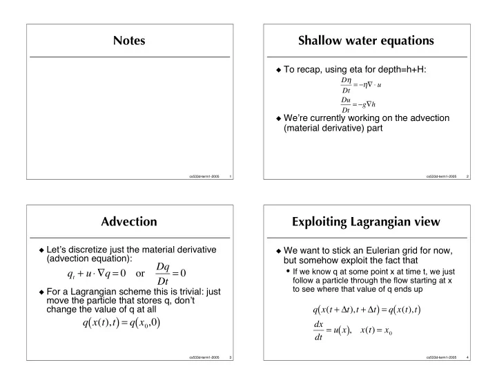
Notes Shallow water equations To recap, using eta for depth=h+H: D Dt = u Du Dt = g h We re currently working on the advection (material derivative) part cs533d-term1-2005 1 cs533d-term1-2005 2
Notes Shallow water equations � To recap, using eta for depth=h+H: D � Dt = � � � � u Du Dt = � g � h � We � re currently working on the advection (material derivative) part cs533d-term1-2005 1 cs533d-term1-2005 2 Advection Exploiting Lagrangian view � Let � s discretize just the material derivative � We want to stick an Eulerian grid for now, (advection equation): but somehow exploit the fact that Dq q t + u � � q = 0 Dt = 0 • If we know q at some point x at time t, we just or follow a particle through the flow starting at x to see where that value of q ends up � For a Lagrangian scheme this is trivial: just move the particle that stores q, don � t ( ) = q x ( t ), t ( ) q x ( t + � t ), t + � t change the value of q at all ( ) = q x 0 ,0 ( ) q x ( t ), t dx ( ) , dt = u x x ( t ) = x 0 cs533d-term1-2005 3 cs533d-term1-2005 4
Looking backwards Semi-Lagrangian method � Problem with tracing particles - we want values at grid � Developed in weather prediction, going back to nodes at the end of the step the 50 � s • Particles could end up anywhere � Also dubbed “stable fluids” in graphics � But… we can look backwards in time (reinvention by Stam � 99) ( ) q ijk = q x ( t � � t ), t � � t � To find new value of q at a grid point, trace particle backwards from grid point (with velocity dx ( ) , dt = u x x ( t ) = x ijk u) for - � t and interpolate from old values of q � Two questions � Same formulas as before - but new interpretation • How do we trace? • To get value of q at a grid point, follow a particle backwards through flow to wherever it started • How do we interpolate? cs533d-term1-2005 5 cs533d-term1-2005 6 Tracing Tracing: 1st order � The errors we make in tracing backwards � We � re at grid node (i,j,k) at position x ijk aren � t too big a deal � Trace backwards through flow for - � t • We don � t compound them - stability isn � t an x old = x ijk � � t u ijk issue • How accurate we are in tracing doesn � t effect • Note - using u value at grid point (what we know shape of q much, just location already) like Forward Euler. � Whether we get too much blurring, oscillations, or � Then can get new q value (with interpolation) a nice result is really up to interpolation n + 1 = q n x old ( ) q ijk � Thus look at “Forward” Euler and RK2 ( ) = q n x ijk � � tu ijk cs533d-term1-2005 7 cs533d-term1-2005 8
Interpolation Linear interpolation � “First” order accurate: nearest neighbour � Error in linear interpolation is proportional to • Just pick q value at grid node closest to x old � x 2 � 2 q • Doesn � t work for slow fluid (small time steps) -- � x 2 nothing changes! � Modified PDE ends up something like… • When we divide by grid spacing to put in terms of ) � x 2 � 2 q Dq advection equation, drops to zero � th order accuracy ( Dt = k � t � x 2 � “Second” order accurate: linear or bilinear (2D) • Ends up first order in advection equation • We have numerical viscosity, things will smear out • Still fast, easy to handle boundary conditions… • For reasonable time steps, k looks like 1/ � t ~ 1/ � x • How well does it work? � [Equivalent to 1st order upwind for CFL � t] � In practice, too much smearing for inviscid fluids cs533d-term1-2005 9 cs533d-term1-2005 10 Nice properties of lerping Cubic interpolation � Linear interpolation is completely stable � To fix the problem of excessive smearing, go to higher order • Interpolated value of q must lie between the old values of q on the grid � E.g. use cubic splines • Thus with each time step, max(q) cannot • Finding interpolating C 2 cubic spline is a little increase, and min(q) cannot decrease painful, an alternative is the � Thus we end up with a fully stable • C 1 Catmull-Rom (cubic Hermite) spline algorithm - take � t as big as you want � [derive] • Great for interactive applications � Introduces overshoot problems • Also simplifies whole issue of picking time • Stability isn � t so easy to guarantee anymore steps cs533d-term1-2005 11 cs533d-term1-2005 12
Min-mod limited Catmull-Rom Back to Shallow Water � See Fedkiw, Stam, Jensen � 01 � So we can now handle advection of both water depth and each component of water � Trick is to check if either slope at the endpoints of the interval has the wrong sign velocity • If so, clamp the slope to zero � Left with the divergence and gradient • Still use cubic Hermite formulas with more reliable terms � � �� � t = � � � u � x + � w slopes � � � This has same stability guarantee as linear � � � z interpolation � u � t = � g � h • But in smoother parts of flow, higher order accurate � x • Called “high resolution” � w � t = � g � h � Still has issues with boundary conditions… � z cs533d-term1-2005 13 cs533d-term1-2005 14 Staggered grid Spatial Discretization � We like central differences - more � So on the MAC grid: accurate, unbiased � � u i + 12 , j � u i � 12 , j + w i , j + 12 � w i , j � 12 � So natural to use a staggered grid for �� ij � t = � � ij � � velocity and height variables � x � z � � • Called MAC grid after the Marker-and-Cell � u i + 12 , j method (Harlow and Welch � 65) that = � g h i + 1, j � h i , j introduced it � t � x � Heights at cell centres � w i , j + 12 = � g h i , j + 1 � h i , j � u-velocities at x-faces of cells � t � z � w-velocities at z-faces of cells cs533d-term1-2005 15 cs533d-term1-2005 16
Solving Full Equations Operator Splitting � Let � s now solve the full incompressible � Generally a bad idea to treat Euler or Navier-Stokes equations incompressible flow as conservation laws with constraints � We � ll first avoid interfaces (e.g. free surfaces) � Instead: split equations up into easy chunks, just like Shallow Water � Think smoke u t + u � � u = 0 u t = � � 2 u u t = g ( ) u t + 1 � � p = 0 � � u = 0 cs533d-term1-2005 17 cs533d-term1-2005 18 Time integration Advection boundary conditions � Don � t mix the steps at all - 1st order accurate � But first, one last issue u (1) = advect ( u n , � t ) � Semi-Lagrangian procedure may need to interpolate from values of u outside the domain, u (2) = u (1) + � � t � 2 u (2) or inside solids u (3) = u (2) + � tg • Outside: no correct answer. Extrapolating from nearest point on domain is fine, or assuming some u n + 1 = u (3) � � t 1 � � p far-field velocity perhaps • Solid walls: velocity should be velocity of wall � We � ve already seen how to do the advection step (e.g.zero) � Often can ignore the second step (viscosity) � Technically only normal component of velocity needs to be � Let � s focus for now on the last step (pressure) taken from wall, in absence of viscosity the tangential component may be better extrapolated from the fluid cs533d-term1-2005 19 cs533d-term1-2005 20
Continuous pressure Pressure boundary conditions � Before we discretize in space, last step is � Issue of what to do for p and u at to take u (3) , figure out the pressure p that boundaries in pressure solve makes u n+1 incompressible: � Think in terms of control volumes: � � u n + 1 = 0 • Want subtract pn from u on boundary so that � � u (3) � � t 1 ( ) = 0 • Plug in pressure update formula: � � p integral of u•n is zero • Rearrange: ( ) = � � u (3) � � � t 1 � � p � So at closed boundary we end up with • Solve this Poisson problem (often density is u n + 1 � n = 0 constant and you can rescale p by it, also � t) � Make this assumption from now on: u n + 1 � n = u (3) � n � � p � 2 p = � � u (3) � n u n + 1 = u (3) � � p cs533d-term1-2005 21 cs533d-term1-2005 22 Pressure BC’s cont’d. Approximate projection � At closed wall boundary have two choices: � Can now directly discretize Poisson equation on a grid � � • Set u•n=0 first, then solve for p with � p/ � n=0, ) ijk = � 2 p � x 2 + � 2 p � y 2 + � 2 p ( � 2 p � � � z 2 � � don � t update velocity at boundary � p i + 1 jk � 2 p ijk + p i � 1 jk + p ij + 1 k � 2 p ijk + p ij � 1 k + p ijk + 1 � 2 p ijk + p ijk � 1 • Or simply solve for p with � p/ � n=u•n and � x 2 � y 2 � z 2 update u•n at boundary with - � p/ � n � � ) ijk = � u � x + � v � y + � w ( � � u � � • Equivalent, but the second option make sense � � z � ijk � u i + 1 jk � u i � 1 jk + v ij + 1 k � v ij � 1 k + w ijk + 1 � w ijk � 1 in the continuous setting, and generally keeps 2 � x 2 � y 2 � z you more honest � � ) ijk � p i + 1 jk � p i � 1 jk , p ij + 1 k � p ij � 1 k , p ijk + 1 � p ijk � 1 ( � p � At open (or free-surface) boundaries, no � � 2 � x 2 � y 2 � z � � constraint on u•n, so typically pick p=0 � Central differences - 2nd order, no bias cs533d-term1-2005 23 cs533d-term1-2005 24
Recommend
More recommend
Explore More Topics
Stay informed with curated content and fresh updates.
