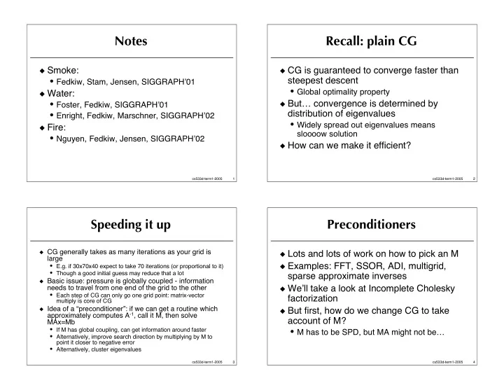
Notes Recall: plain CG Smoke: CG is guaranteed to converge faster - PowerPoint PPT Presentation

Notes Recall: plain CG � Smoke: � CG is guaranteed to converge faster than steepest descent • Fedkiw, Stam, Jensen, SIGGRAPH � 01 • Global optimality property � Water: • Foster, Fedkiw, SIGGRAPH � 01 � But… convergence is determined by distribution of eigenvalues • Enright, Fedkiw, Marschner, SIGGRAPH � 02 • Widely spread out eigenvalues means � Fire: sloooow solution • Nguyen, Fedkiw, Jensen, SIGGRAPH � 02 � How can we make it efficient? cs533d-term1-2005 1 cs533d-term1-2005 2 Speeding it up Preconditioners � CG generally takes as many iterations as your grid is � Lots and lots of work on how to pick an M large � Examples: FFT, SSOR, ADI, multigrid, • E.g. if 30x70x40 expect to take 70 iterations (or proportional to it) • Though a good initial guess may reduce that a lot sparse approximate inverses � Basic issue: pressure is globally coupled - information � We � ll take a look at Incomplete Cholesky needs to travel from one end of the grid to the other • Each step of CG can only go one grid point: matrix-vector factorization multiply is core of CG � Idea of a “preconditioner”: if we can get a routine which � But first, how do we change CG to take approximately computes A -1 , call it M, then solve account of M? MAx=Mb • If M has global coupling, can get information around faster • M has to be SPD, but MA might not be… • Alternatively, improve search direction by multiplying by M to point it closer to negative error • Alternatively, cluster eigenvalues cs533d-term1-2005 3 cs533d-term1-2005 4

PCG Cholesky � r=b-Ap, z=Mr, s=z � True Gaussian elimination, which is called � � =z T r, check if already solved Cholesky factorization in the SPD case, gives A=LL T � Loop: • t=As � L is a lower triangular matrix • � = � /(s T t) � Then solving Ap=b can be done by • x+= � s, r-= � t , check for convergence • Lx=p, L T p=x • z=Mr • Each solve is easy to do - triangular • � new =z T r • � = � new / � � But can � t do that here since L has many more • s=z+ � s nonzeros than A -- EXPENSIVE! • � = � new cs533d-term1-2005 5 cs533d-term1-2005 6 Incomplete Cholesky IC(0) � We only need approximate result for preconditioner � Incomplete Cholesky level 0: IC(0) is where we � So do Cholesky factorization, but throw away new make sure L=0 wherever A=0 nonzeros (set them to zero) � For this A (7-point Laplacian) with the regular � Result is not exact, but pretty good grid ordering, things are nice • Instead of O(n) iterations (for an n 3 grid) we get O(n 1/2 ) iterations � Can actually do better: � Write A=F+D+F T where F is strictly lower • Modified Incomplete Cholesky triangular and D is diagonal • Same algorithm, only when we throw away nonzeros, we add them to the diagonal - better behaviour with low frequency � Then IC(0) ends up being of the form components of pressure L=(FE -1 +E) where E is diagonal • Gets us down to O(n 1/4 ) iterations • We only need to compute and store E! cs533d-term1-2005 7 cs533d-term1-2005 8

Computing IC(0) Diagonal Entry � Need to find diagonal E so that (LL T ) ij =A ij � Assume we order increasing in i, j, k wherever A ij � 0 � Note F=A for lower diagonal elements � Expand out: ( ) ijk , ijk = E ijk 2 + A ijk , i � 1 jk + A ijk , ij � 1 k + A ijk , ijk � 1 T 2 2 2 2 2 2 LL E i � 1 jk E ij � 1 k E ijk � 1 • LL T =F+F T +E 2 +FE -2 F T � Again, for this special case, can show that last � Want this to match A � s diagonal term only contributes to diagonal and elements Then solving for next E ijk in terms of where A ij =0 previously determined ones: � So we get the off-diagonal correct for free � Let � s take a look at diagonal entry for grid point E ijk = A ijk , ijk � A ijk , i � 1 jk � A ijk , ij � 1 k � A ijk , ijk � 1 2 2 2 2 2 2 E i � 1 jk E ij � 1 k E ijk � 1 ijk cs533d-term1-2005 9 cs533d-term1-2005 10 Practicalities Viscosity � Actually only want to store inverse of E � The viscosity update (if we really need it - highly viscous fluids) is just Backwards Euler: � Note that for values of A or E off the grid, ( ) u (3) = u (2) substitute zero in formula I � � t � � 2 • In particular, can start at E 000,000 = � A 000,000 � Boils down to almost the same linear system to � Modified Incomplete Cholesky looks very similar, solve! except instead of matching diagonal entries, we match row sums • Or rather, 3 similar linear systems to solve - one for each component of velocity � Can squeeze out a little more performance with (NOTE: solve separately, not together!) the “Eisenstat trick” • Again use PCG with Incomplete Cholesky cs533d-term1-2005 11 cs533d-term1-2005 12

Staggered grid advection Vorticity confinement � The interpolation errors behave like � Problem: velocity on a staggered grid, don � t have components where we need it for semi-Lagrangian steps viscosity, the averaging from the � Simple answer staggered grid behaves like viscosity… • Average velocities to get flow field where you need it, e.g. • Net effect is that interesting flow structures u ijk =0.5(u i+1/2 jk + u i-1/2 jk ) (vortices) get smeared out • So advect each component of velocity around in averaged velocity field � Idea of vorticity confinement - add a fake � Even cheaper force that spins vortices faster • Advect averaged velocity field around (with any other quantity • Compute vorticity of flow, add force in you care about) --- reuse interpolation coefficients! direction of flow around each vortex • But - all that averaging smears u out… more numerical viscosity! • Try to cancel off some of the numerical [worse for small � t] viscosity in a stable way cs533d-term1-2005 13 cs533d-term1-2005 14 Smoke Smoke concentration � Smoke is a bit more than just a velocity field � There � s more than just air temperature to consider too � Need temperature (hot air rises) and smoke density (smoke eventually falls) � Smoke weighs more than air - so need to track � Real physics - density depends on temperature, smoke concentration temperature depends on viscosity and thermal • Also could be used for rendering (though tracing conduction, … particles can give better results) • We � ll ignore most of that: small scale effects • Point is: physics depends on smoke concentration, • Boussinesq approximation: ignore density variation except in not just appearance gravity term, ignore energy transfer except thermal conduction • We might go a step further and ignore thermal conduction - � We again ignore effect of this in all terms except insignificant vs. numerical dissipation - but we � re also ignoring gravity force sub-grid turbulence which is really how most of the temperature gets diffused cs533d-term1-2005 15 cs533d-term1-2005 16

Buoyancy Smoke equations � So putting it all together… � For smoke, where there is no interface, we can add � gy to pressure (and just solve for the ( ) (0,1,0) u t + u � � u + � p = � � s + � T difference) thus cancelling out g term in equation � � u = 0 � All that � s left is buoyancy -- variation in vertical force due to density variation T t + u � � T = k � 2 T � Density varies because of temperature change s t + u � � s = 0 and because of smoke concentration � We know how to solve the u part, using old � Assume linear relationship (small variations) ( ) f bouy = � � s + � T values for s and T � Advecting s and T around is simple - just scalar • T=0 is ambient temperature; � , � depend on g etc. advection � Heat diffusion handled like viscosity cs533d-term1-2005 17 cs533d-term1-2005 18 Notes on discretization Water � Smoke concentration and temperature may as well live in grid cells same as pressure � But then to add buoyancy force, need to average to get values at staggered positions � Also, to maintain conservation properties, should only advect smoke concentration and temperature (and anything else - velocity) in a divergence-free velocity field • If you want to do all the advection together, do it before adding buoyancy force • I.e. advect; buoyancy; pressure solve; repeat cs533d-term1-2005 19 cs533d-term1-2005 20

Water - Free Surface Flow Interface Velocity � Chief difference: instead of smoke density � Fluid interface moves with the velocity of and temperature, need to track a free the fluid at the interface surface • Technically only need the normal component of that motion… � If we know which grid cells are fluid and � To help out algorithms, usually want to which aren � t, we can apply p=0 boundary extrapolate velocity field out beyond free condition at the right grid cell faces surface • First order accurate… � Main problem: tracking the surface effectively cs533d-term1-2005 21 cs533d-term1-2005 22 Marker Particle Issues Issues � From the original MAC paper (Harlow + � Very simple to implement, fairly robust Welch � 65) � Hard to determine a smooth surface for � Start with several particles per grid cell rendering (or surface tension!) � After every step (updated velocity) move • Blobbies look bumpy, stair step grid version is particles in the velocity field worse • dx/dt=u(x) • But with enough post-smoothing, ok for • Probably advisable to use at least RK2 anything other than really smooth flow � At start of next step, identify grid cells containing at least one particle: this is where the fluid is cs533d-term1-2005 23 cs533d-term1-2005 24