Non-homogeneous incompressible Bingham flows with variable yield - PowerPoint PPT Presentation
Non-homogeneous incompressible Bingham flows with variable yield stress and application to volcanology. Jordane Math with Laurent Chupin (maths) and Karim Kelfoun (LMV) Laboratoire de Maths & Laboratoire Magmas et Volcans june 2015 Jordane
Non-homogeneous incompressible Bingham flows with variable yield stress and application to volcanology. Jordane Mathé with Laurent Chupin (maths) and Karim Kelfoun (LMV) Laboratoire de Maths & Laboratoire Magmas et Volcans june 2015 Jordane Mathé (Maths-LMV) Fluidized granular flows june 2015 1 / 18
Jordane Mathé (Maths-LMV) Fluidized granular flows june 2015 2 / 18
Laboratory experiment Zoom into the granular column → O. Roche , LMV. Jordane Mathé (Maths-LMV) Fluidized granular flows june 2015 3 / 18
Laboratory experiment Zoom into the granular column → Fluidisation : injection of gas through a pore plate. O. Roche , LMV. Jordane Mathé (Maths-LMV) Fluidized granular flows june 2015 3 / 18
Figure: Non-fluidised → short runout distance Figure: Fluidised → long runout distance
Model 1 Numerical simulation 2 Perspectives 3 Jordane Mathé (Maths-LMV) Fluidized granular flows june 2015 5 / 18
Model 1 Jordane Mathé (Maths-LMV) Fluidized granular flows june 2015 6 / 18
Two phases for one fluid Consider one mixed fluid with variable density .
Two phases for one fluid Consider one mixed fluid with variable density . It satisfies the non-homogeneous incompressible Navier-Stokes equations: div ( v ) = 0 ∂ t ρ + div ( ρ v ) = 0 ∂ t ( ρ v ) + div ( ρ v ⊗ v ) + ∇ p = ρ g + div ( S )
Two phases for one fluid Consider one mixed fluid with variable density . It satisfies the non-homogeneous incompressible Navier-Stokes equations: div ( v ) = 0 ∂ t ρ + div ( ρ v ) = 0 ∂ t ( ρ v ) + div ( ρ v ⊗ v ) + ∇ p = ρ g + div ( S ) Unknown: v : velocity, p : total pressure, ρ : density.
Two phases for one fluid Consider one mixed fluid with variable density . It satisfies the non-homogeneous incompressible Navier-Stokes equations: div ( v ) = 0 ∂ t ρ + div ( ρ v ) = 0 ∂ t ( ρ v ) + div ( ρ v ⊗ v ) + ∇ p = ρ g + div ( S ) Constant g : gravity.
Two phases for one fluid Consider one mixed fluid with variable density . It satisfies the non-homogeneous incompressible Navier-Stokes equations: div ( v ) = 0 ∂ t ρ + div ( ρ v ) = 0 ∂ t ( ρ v ) + div ( ρ v ⊗ v ) + ∇ p = ρ g + div ( S ) Constant g : gravity. Rheology Let precise S .
Rheology In our case S = µ Dv + Dv = ˙ γ is the strain rate tensor, where µ is the effective viscosity
Rheology In our case S = µ Dv + Σ , Dv = ˙ γ is the strain rate tensor, Σ = q Dv where µ is the effective viscosity | Dv | ⇒ Bingham fluid with yield stress q
Rheology In our case S = µ Dv + Σ , Dv = ˙ γ is the strain rate tensor, Σ = q Dv where µ is the effective viscosity | Dv | ⇒ Bingham fluid with yield stress q Idea Let vary the yield stress q as a function of the interstitial gas pressure .
Variation of the yield stress Definition of the yield stress � atmospheric pressure: Coulomb friction = q high pressure: fluid Jordane Mathé (Maths-LMV) Fluidized granular flows june 2015 9 / 18
Variation of the yield stress Definition of the yield stress � atmospheric pressure: Coulomb friction = q high pressure: fluid � tan( δ )( ρ gh − gas pressure) if low gas pressure = q 0 if high gas pressure where δ is the internal friction angle. Jordane Mathé (Maths-LMV) Fluidized granular flows june 2015 9 / 18
Variation of the yield stress Definition of the yield stress � atmospheric pressure: Coulomb friction = q high pressure: fluid � tan( δ )( ρ gh − gas pressure) if low gas pressure = q 0 if high gas pressure tan( δ )( ρ gh − gas pressure) + = q where δ is the internal friction angle. Jordane Mathé (Maths-LMV) Fluidized granular flows june 2015 9 / 18
Equations of the model Noting p f the interstitial gas pressure, we obtain: div ( v ) = 0 ∂ t ρ + div ( ρ v ) = 0 Dv ( ρ gh − p f ) + + ρ g ∂ t ( ρ v ) + div ( ρ v ⊗ v ) − µ ∆ v + ∇ p = tan( δ ) div � �� � | Dv | yield q
Equations of the model Noting p f the interstitial gas pressure, we obtain: div ( v ) = 0 ∂ t ρ + div ( ρ v ) = 0 Dv ( ρ gh − p f ) + + ρ g ∂ t ( ρ v ) + div ( ρ v ⊗ v ) − µ ∆ v + ∇ p = tan( δ ) div � �� � | Dv | yield q ∂ t p f + v · ∇ p f − κ ∆ p f = 0 where κ is the diffusion coefficient.
Numerical simulation 2 Jordane Mathé (Maths-LMV) Fluidized granular flows june 2015 11 / 18
Dambreak: Mesh Jordane Mathé (Maths-LMV) Fluidized granular flows june 2015 12 / 18
Dambreak: how to treat the density? ∂ t ρ + v · ∇ ρ = 0 numerical method: RK3 TVD - WENO5 scheme. Jordane Mathé (Maths-LMV) Fluidized granular flows june 2015 12 / 18
Numerical scheme (without density) v 0 , Σ 0 , p 0 and p f 0 given. n = 0
Numerical scheme (without density) v 0 , Σ 0 , p 0 and p f 0 given. n = 0 v n , Σ n , p n and p f n being calculated. n � 0
Numerical scheme (without density) v 0 , Σ 0 , p 0 and p f 0 given. n = 0 v n , Σ n , p n and p f n being calculated. n � 0 v n +1 , Σ n +1 ) solution of We compute ( � v n +1 − 4 v n + v n − 1 v n +1 ρ n +1 = div Σ n +1 3 � + 2 v n ·∇ v n − v n − 1 ·∇ v n − 1 − ∆ � + ∇ p n − e y , ρ n +1 ρ n +1 2 δ t Σ n +1 = P q n (Σ n +1 + r D � v n +1 + ε (Σ n − Σ n +1 )) , v n +1 � � � = 0 . � ∂ Ω
Numerical scheme (without density) v 0 , Σ 0 , p 0 and p f 0 given. n = 0 v n , Σ n , p n and p f n being calculated. n � 0 v n +1 , Σ n +1 ) solution of We compute ( � v n +1 − 4 v n + v n − 1 v n +1 ρ n +1 = div Σ n +1 3 � + 2 v n ·∇ v n − v n − 1 ·∇ v n − 1 − ∆ � + ∇ p n − e y , ρ n +1 ρ n +1 2 δ t Σ n +1 = P q n (Σ n +1 + r D � v n +1 + ε (Σ n − Σ n +1 )) , v n +1 � � � = 0 . � ∂ Ω We compute ( v n +1 , p n +1 ) thanks to the incompressibility constrain v n +1 − � v n +1 2 3 ρ n +1 ∇ ( p n +1 − p n ) = 0 , + δ t � � div v n +1 = 0 , v n +1 · n ∂ Ω = 0 . �
Numerical scheme (without density) v 0 , Σ 0 , p 0 and p f 0 given. n = 0 v n , Σ n , p n and p f n being calculated. n � 0 v n +1 , Σ n +1 ) solution of We compute ( � v n +1 − 4 v n + v n − 1 v n +1 ρ n +1 = div Σ n +1 3 � + 2 v n ·∇ v n − v n − 1 ·∇ v n − 1 − ∆ � + ∇ p n − e y , ρ n +1 ρ n +1 2 δ t Σ n +1 = P q n (Σ n +1 + r D � v n +1 + ε (Σ n − Σ n +1 )) , v n +1 � � � = 0 . � ∂ Ω We compute ( v n +1 , p n +1 ) thanks to the incompressibility constrain v n +1 − � v n +1 2 3 ρ n +1 ∇ ( p n +1 − p n ) = 0 , + δ t � � div v n +1 = 0 , v n +1 · n ∂ Ω = 0 . � We compute p f n +1 solution of 3 p f n +1 − 4 p f n + p f n − 1 + 2 v n +1 · ∇ p f n − v n +1 · ∇ p f n − 1 − ∆ p f n +1 = 0 . 2 δ t
Numerical scheme (without density) v 0 , Σ 0 , p 0 and p f 0 given. n = 0 v n , Σ n , p n and p f n being calculated. n � 0 v n +1 , Σ n +1 ) solution of We compute ( � v n +1 − 4 v n + v n − 1 v n +1 ρ n +1 = div Σ n +1 3 � + 2 v n ·∇ v n − v n − 1 ·∇ v n − 1 − ∆ � + ∇ p n − e y , ρ n +1 ρ n +1 2 δ t Σ n +1 = P q n (Σ n +1 + r D � v n +1 + ε (Σ n − Σ n +1 )) , v n +1 � � � = 0 . � ∂ Ω Σ n , 0 = Σ n , and ( v n , p n , p n ֒ → k = 0 f ) given. Σ n , k known, we first compute � v n , k solution of a → k � 0 ֒ Laplace-type problem then we project the stress tensor to obtain Σ n , k +1 : v n , k − 4 v n + v n − 1 ρ n +1 + ∇ p n v n , k ρ n +1 = div Σ n , k 3 � + 2 v n ·∇ v n − v n − 1 ·∇ v n − 1 − ∆ � − e y , 2 δ t ρ n +1 v n , k � � � = 0 , � ∂ Ω Σ n , k +1 = P q n (Σ n , k + r D � v n , k + ε (Σ n − Σ n , k )) .
Numerical scheme (without density) v 0 , Σ 0 , p 0 and p f 0 given. n = 0 v n , Σ n , p n and p f n being calculated. n � 0 v n +1 , Σ n +1 ) solution of We compute ( � v n +1 − 4 v n + v n − 1 v n +1 ρ n +1 = div Σ n +1 3 � + 2 v n ·∇ v n − v n − 1 ·∇ v n − 1 − ∆ � + ∇ p n − e y , ρ n +1 ρ n +1 2 δ t Σ n +1 = P q n (Σ n +1 + r D � v n +1 + ε (Σ n − Σ n +1 )) , v n +1 � � � = 0 . � ∂ Ω Σ n , 0 = Σ n , and ( v n , p n , p n ֒ → k = 0 f ) given. Σ n , k known, we first compute � v n , k solution of a → k � 0 ֒ Laplace-type problem then we project the stress tensor to obtain Σ n , k +1 : v n , k − 4 v n + v n − 1 ρ n +1 + ∇ p n v n , k ρ n +1 = div Σ n , k 3 � + 2 v n ·∇ v n − v n − 1 ·∇ v n − 1 − ∆ � − e y , 2 δ t ρ n +1 v n , k � � � = 0 , � ∂ Ω Σ n , k +1 = P q n (Σ n , k + r D � v n , k + ε (Σ n − Σ n , k )) .
Recommend
More recommend
Explore More Topics
Stay informed with curated content and fresh updates.
