Natural Language Understanding Lecture 11: Unsupervised - PowerPoint PPT Presentation
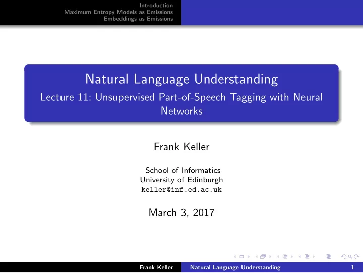
Introduction Maximum Entropy Models as Emissions Embeddings as Emissions Natural Language Understanding Lecture 11: Unsupervised Part-of-Speech Tagging with Neural Networks Frank Keller School of Informatics University of Edinburgh
Introduction Maximum Entropy Models as Emissions Embeddings as Emissions Natural Language Understanding Lecture 11: Unsupervised Part-of-Speech Tagging with Neural Networks Frank Keller School of Informatics University of Edinburgh keller@inf.ed.ac.uk March 3, 2017 Frank Keller Natural Language Understanding 1
Introduction Maximum Entropy Models as Emissions Embeddings as Emissions 1 Introduction Hidden Markov Models Extending HMMs 2 Maximum Entropy Models as Emissions Estimation Features Results 3 Embeddings as Emissions Embeddings Estimation Results Reading: Berg-Kirkpatrick et al. (2010); Lin et al. (2015). Background: Jurafsky and Martin (2009: Ch. 6.5). Frank Keller Natural Language Understanding 2
Introduction Hidden Markov Models Maximum Entropy Models as Emissions Extending HMMs Embeddings as Emissions Hidden Markov Models Recall our notation for HMM from the last lecture: ����� � ���� � �� � ��� � � ���� ������ � ���� � �� � ��� ��� �� �� n � P ( t , w ) = P ( t i | t i − 1 ) P ( w i | t i ) i =1 The parameters of the HMM are θ = ( τ, ω ). They define: τ : the probability distribution over tag-tag transitions; ω : the probability distribution over word-tag outputs. Frank Keller Natural Language Understanding 3
Introduction Hidden Markov Models Maximum Entropy Models as Emissions Extending HMMs Embeddings as Emissions Hidden Markov Models The model is based on a set of multinomial distributions. For tag types t = 1 . . . T and word types w = 1 . . . W : ω = ω (1) . . . ω ( T ) : the output distributions for each tag; τ = τ (1) . . . τ ( T ) : the transition distributions for each tag; ω ( t ) = ω ( t ) 1 . . . ω ( t ) W : the output distribution from tag t ; τ ( t ) = τ ( t ) . . . τ ( t ) T : the transition distribution from tag t . 1 Goal of this lecture: replace the output distributions ω with something cleverer than multinomials. Frank Keller Natural Language Understanding 4
Introduction Hidden Markov Models Maximum Entropy Models as Emissions Extending HMMs Embeddings as Emissions Hidden Markov Models Example: ω ( NN ) is the output distribution for tag NN : w John Mary running jumping [Source: Taylor Berg-Kirkpatrick et al: Painless Unsupervised Learning with Features, ACL slides 2010.] Frank Keller Natural Language Understanding 5
Introduction Hidden Markov Models Maximum Entropy Models as Emissions Extending HMMs Embeddings as Emissions Hidden Markov Models Example: ω ( NN ) is the output distribution for tag NN : ω ( NN ) w w 0.1 John 0.0 Mary 0.2 running 0.0 jumping [Source: Taylor Berg-Kirkpatrick et al: Painless Unsupervised Learning with Features, ACL slides 2010.] Frank Keller Natural Language Understanding 5
Introduction Hidden Markov Models Maximum Entropy Models as Emissions Extending HMMs Embeddings as Emissions Hidden Markov Models Example: ω ( NN ) is the output distribution for tag NN : ω ( NN ) w f ( NN , w ) w 0.1 John +Cap 0.0 Mary +Cap 0.2 running +ing 0.0 jumping +ing [Source: Taylor Berg-Kirkpatrick et al: Painless Unsupervised Learning with Features, ACL slides 2010.] Frank Keller Natural Language Understanding 5
Introduction Hidden Markov Models Maximum Entropy Models as Emissions Extending HMMs Embeddings as Emissions Hidden Markov Models Example: ω ( NN ) is the output distribution for tag NN : ω ( NN ) e λ · f ( NN , w ) w f ( NN , w ) w 0.1 John +Cap 0.3 0.0 Mary +Cap 0.3 0.2 running +ing 0.1 0.0 jumping +ing 0.1 First idea: use local features to define ω ( t ) (Berg-Kirkpatrick et al. 2010): exp( λ · f ( t , w )) ω ( t ) w = (1) w ′ exp( λ · f ( t , w ′ )) � Multinomials become maximum entropy models. [Source: Taylor Berg-Kirkpatrick et al: Painless Unsupervised Learning with Features, ACL slides 2010.] Frank Keller Natural Language Understanding 5
Introduction Hidden Markov Models Maximum Entropy Models as Emissions Extending HMMs Embeddings as Emissions Hidden Markov Models Example: ω ( NN ) is the output distribution for tag NN : w John Mary running jumping Frank Keller Natural Language Understanding 6
Introduction Hidden Markov Models Maximum Entropy Models as Emissions Extending HMMs Embeddings as Emissions Hidden Markov Models Example: ω ( NN ) is the output distribution for tag NN : ω ( NN ) w w 0.1 John 0.0 Mary 0.2 running 0.0 jumping Frank Keller Natural Language Understanding 6
Introduction Hidden Markov Models Maximum Entropy Models as Emissions Extending HMMs Embeddings as Emissions Hidden Markov Models Example: ω ( NN ) is the output distribution for tag NN : ω ( NN ) w v w w 0.1 John [0 . 1 0 . 4 0 . 06 1 . 7] 0.0 Mary [0 . 2 1 . 3 0 . 20 0 . 0] 0.2 running [3 . 1 0 . 4 0 . 06 1 . 7] 0.0 jumping [0 . 7 0 . 4 0 . 02 0 . 5] Frank Keller Natural Language Understanding 6
Introduction Hidden Markov Models Maximum Entropy Models as Emissions Extending HMMs Embeddings as Emissions Hidden Markov Models Example: ω ( NN ) is the output distribution for tag NN : ω ( NN ) p ( v w ; µ t , Σ t ) w v w w 0.1 John [0 . 1 0 . 4 0 . 06 1 . 7] 0.3 0.0 Mary [0 . 2 1 . 3 0 . 20 0 . 0] 0.3 0.2 running [3 . 1 0 . 4 0 . 06 1 . 7] 0.1 0.0 jumping [0 . 7 0 . 4 0 . 02 0 . 5] 0.1 Second idea: use word embeddings to define ω ( t ) (Lin et al. 2015): w = exp( − 1 2 ( v w − µ t ) ⊤ Σ − 1 t ( v w − µ t )) ω ( t ) � (2 π ) d | Σ t | Multinomials become multivariate Gaussians with d dimensions. Frank Keller Natural Language Understanding 6
Introduction Estimation Maximum Entropy Models as Emissions Features Embeddings as Emissions Results Standard Expectation Maximization For both ideas, we can use the Expectation Maximization Algorithm to estimate model parameters. Standard EM optimizes L ( θ ) = log P θ ( w ). The E-step computes the expected counts for the emissions: �� � � � e ( t , w ) ← E ω I ( t , w i ) � w (2) � i The expected counts are then normalized in the M-step to re-estimate θ : e ( t , w ) ω ( t ) w ← (3) � w ′ e ( t , w ′ ) The expected counts can be computed efficiently using the Forward-Backward algorithm (aka Baum-Welch algorithm). Frank Keller Natural Language Understanding 7
Introduction Estimation Maximum Entropy Models as Emissions Features Embeddings as Emissions Results Expectation Maximization for HMMs with Features Now the E-step first computes ω ( t ) given λ as in (1), then it w computes the expectations as in (2) using Forward-Backward. The M-step now optimizes the regularized expected log likelihood over all word-tag pairs: e ( t , w ) log ω ( t ) � w ( λ ) − κ || λ || 2 ℓ ( λ , e ) = 2 ( t , w ) To compute ℓ ( λ , e ), we use a general gradient-based search algorithm, e.g., the LBFGS (Limited-memory Broyden-Fletcher- Goldfarb-Shanno) algorithm. Frank Keller Natural Language Understanding 8
Introduction Estimation Maximum Entropy Models as Emissions Features Embeddings as Emissions Results HMMs with Features The key advantage of Berg-Kirkpatrick et al.’s (2010) approach is that we can now add arbitrary features to the HMM: BASIC: I ( w = · , t = · ) CONTAINS-DIGIT: Check if w contains digit and conjoin with t : I ( containsDigit ( w ) = · , t = · ) CONTAINS-HYPHEN: I ( containsHyphen ( w ) = · , t = · ) INITIAL-CAP: Check if the first letter of w is capitalized: I ( isCap ( w ) = · , t = · ) N-GRAM: Indicator functions for character n-grams of up to length 3 present in w . A standard HMM only has the BASIC features. ( I is the indicator function; returns 1 if the features is present, 0 otherwise.) Frank Keller Natural Language Understanding 9
Introduction Estimation Maximum Entropy Models as Emissions Features Embeddings as Emissions Results Results 56.0 +12.8 43.2 Basic Multinomial: Rich Features: John ∧ NNP John ∧ NNP +Digit ∧ NNP +Hyph ∧ NNP +Cap ∧ NNP +ing ∧ NNP [Source: Taylor Berg-Kirkpatrick et al: Painless Unsupervised Learning with Features, ACL slides 2010.] Frank Keller Natural Language Understanding 10
Introduction Embeddings Maximum Entropy Models as Emissions Estimation Embeddings as Emissions Results Embeddings as Multivariate Gaussians Given a tag t , instead of a word w , we generate a pretrained embedding v w ∈ R d ( d dimensionality of the embedding). We assume that v w is distributed according to a multivariate Gaussian with the mean vector µ t and covariance matrix Σ t : w = p ( v w ; µ t , Σ t ) = exp( − 1 2 ( v w − µ t ) ⊤ Σ − 1 t ( v w − µ t )) ω ( t ) � (2 π ) d | Σ t | This means we assume that the embeddings of words which are often tagged as t are concentrated around the point µ t , where the concentration decays according to Σ t . Frank Keller Natural Language Understanding 11
Introduction Embeddings Maximum Entropy Models as Emissions Estimation Embeddings as Emissions Results Embeddings as Multivariate Gaussians Now, the joint distribution over a sequence of words w = w 1 . . . w n is represented as a sequence of vectors v = v w 1 . . . v w n . The joint probability of a word and tag sequence is: n � P ( t , w ) = P ( t i | t i − 1 ) p ( v w ; µ t , Σ t ) i =1 We again estimate the parameters µ t and Σ t using Forward-Backward. Frank Keller Natural Language Understanding 12
Recommend
More recommend
Explore More Topics
Stay informed with curated content and fresh updates.
