n ( n ( I ( i , j ) = i j minimize ... | {z } r r . . - PowerPoint PPT Presentation
Spacetime least-squares PetrovGalerkin projection for nonlinear model reduction r ) + r ( P k minimize r ( v ; ) k 2 P r r v n ( n ( I ( i , j ) = i j minimize ... | {z } r r . .
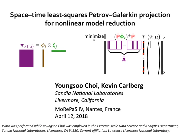
Space–time least-squares Petrov–Galerkin projection for nonlinear model reduction Φ r ) + ¯ r (¯ P ¯ k minimize r (ˆ v ; µ ) k 2 P¯ r ¯ r ¯ ˆ v n ( n ( π I ( i , j ) = φ i ⊗ ξ j minimize ... | {z } r r . ¯ . A . k 2 Youngsoo Choi, Kevin Carlberg Sandia Na(onal Laboratories Livermore, California MoRePaS IV, Nantes, France April 12, 2018 Work was performed while Youngsoo Choi was employed in the Extreme-scale Data Science and Analy(cs Department, Sandia Na(onal Laboratories, Livermore, CA 94550. Current affilia(on: Lawrence Livermore Na(onal Laboratory.
Motivation d x ODE: x (0, µ ) = x 0 ( µ ), dt = f ( x ; t , µ ); t ∈ [0, T final ] , µ ∈ D O∆E: r n ( x n , ... , x n − k ; µ ) = 0 , final ] , n = 1, ... , T µ ∈ D number of Dme steps T state variables N number of 2 Space–8me least-squares Petrov–Galerkin projec8on Choi and Carlberg
Motivation d x ODE: x (0, µ ) = x 0 ( µ ), dt = f ( x ; t , µ ); t ∈ [0, T final ] , µ ∈ D O∆E: r n ( x n , ... , x n − k ; µ ) = 0 , final ] , n = 1, ... , T µ ∈ D number of Dme steps T state variables N number of Most ROMs for nonlinear dynamical systems use spa(al simula(on data to reduce the spa(al dimension and complexity 2 Space–8me least-squares Petrov–Galerkin projec8on Choi and Carlberg
Motivation d x ODE: x (0, µ ) = x 0 ( µ ), dt = f ( x ; t , µ ); t ∈ [0, T final ] , µ ∈ D O∆E: r n ( x n , ... , x n − k ; µ ) = 0 , final ] , n = 1, ... , T µ ∈ D number of Dme steps T state variables N number of Most ROMs for nonlinear dynamical systems use spa(al simula(on data to reduce the spa(al dimension and complexity Goal: use temporal simula/on data to reduce the temporal dimension and complexity 2 Space–8me least-squares Petrov–Galerkin projec8on Choi and Carlberg
Offline step 1 : data collection O∆E: r n ( x n , ... , x n − k ; µ ) = 0 , n = 1, ... , T number of Dme steps T state variables N number of D 3 Space–8me least-squares Petrov–Galerkin projec8on Choi and Carlberg
Offline step 1 : data collection O∆E: r n ( x n , ... , x n − k ; µ ) = 0 , n = 1, ... , T X = D 3 Space–8me least-squares Petrov–Galerkin projec8on Choi and Carlberg
Offline step 2: Tensor decomposition (POD) O∆E: r n ( x n , ... , x n − k ; µ ) = 0 , n = 1, ... , T Compute dominant leP singular vectors of mode-1 unfolding V T X (1) = U Σ X = = �4 Space–8me least-squares Petrov–Galerkin projec8on Choi and Carlberg
Offline step 2: Tensor decomposition (POD) O∆E: r n ( x n , ... , x n − k ; µ ) = 0 , n = 1, ... , T Compute dominant leP singular vectors of mode-1 unfolding V T X (1) = Φ U Σ X = = columns are principal components of the spa(al simula(on data Φ �4 Space–8me least-squares Petrov–Galerkin projec8on Choi and Carlberg
Online : LSPG projection [C., Bou–Mosleh, Farhat, 2011] O∆E: r n ( x n , ... , x n − k ; µ ) = 0 , n = 1, ... , T D 1. Reduce number of spaDal unknowns 2. Minimize O∆E residual x n = Φ ˆ x n ≈ ˜ x n = arg min x n � � x n − 1 , ... , ˜ x n − k ; µ ) � Ar n ( Φ ˆ ˆ v , ˜ � � � 2 ˆ v ( ( 2 2 x n = arg min � Ar n ( x 0 + Φ ˆ � � LSPG O∆E: ˆ x n − 1 , ... , ˜ x n − k ; µ ) v , ˜ D � � � 2 ˆ v 5 Space–8me least-squares Petrov–Galerkin projec8on Choi and Carlberg
Ahmed body [Ahmed, Ramm, Faitin, 1984] V ∞ ‣ Unsteady Navier–Stokes ‣ M ∞ = 0.175 ‣ Re = 4.3 x 10 6 Spa8al discre8za8on Temporal discre8za8on ‣ 2nd-order finite volume ‣ 2nd-order BDF ‣ DES turbulence model ‣ Time step ∆ t = 8 × 10 − 5 s ‣ degrees of freedom ‣ Dme instances 1.3 × 10 3 1.7 × 10 7 6 Space–8me least-squares Petrov–Galerkin projec8on Choi and Carlberg
Ahmed body results [C., Farhat, Cortial, Amsallem, 2013] high-fidelity model GNAT ROM ( kjsdfskjdkjkkj) A = ( P Φ r ) + P 13 hours, 512 cores 4 hours, 4 cores spa(al dim : 283 spa(al dim : 1.7 x 10 7 temporal dim : 1.3 x 10 3 temporal dim : 1.3 x 10 3 pressure field + 438X computa(onal-cost reduc(on + 60,500X spa(al-dimension reduc(on - Zero temporal-dimension reduc(on 7 Space–8me least-squares Petrov–Galerkin projec8on Choi and Carlberg
B61 captive carry V ∞ ‣ Unsteady Navier–Stokes ‣ Re = 6.3 x 10 6 ‣ M ∞ = 0.6 Spa8al discre8za8on Temporal discre8za8on ‣ 2nd-order finite volume ‣ 2nd-order BDF ‣ DES turbulence model ‣ Verified Dme step ∆ t = 1.5 × 10 − 3 ‣ degrees of freedom ‣ Dme instances 1.2 × 10 6 8.3 × 10 3 8 Space–8me least-squares Petrov–Galerkin projec8on Choi and Carlberg
Turbulent-cavity results [C., Barone, Antil, 2017] vor(city field pressure field GNAT ROM 32 min, 2 cores spa(al dim : 179 temporal dim : 458 high-fidelity 5 hours, 48 cores spa(al dim : 1.2M temporal dim : 3,700 + 229X computa(onal-cost reduc(on + 6,500X spa(al-dimension reduc(on - 8X temporal-dimension reduc(on How can we significantly reduce the temporal dimensionality? 9 Space–8me least-squares Petrov–Galerkin projec8on Choi and Carlberg
Reducing temporal complexity : existing work Larger 8me steps with ROM [Krysl et al., 2001; Lucia et al., 2004; Taylor et al., 2010; C. et al., 2017] ‣ Developed for explicit and implicit integrators - Limited reducDon of Dme dimension: <10X reducDons typical Forecas8ng using gappy POD in 8me ‣ Accurate Newton-solver iniDal guess [C., Ray, van Bloemen Waanders, 2015] ‣ Coarse propagator in Dme-parallel sekng [C., Brencher, Haasdonk, Barth, 2016] + No error incurred and wall-Dme improvements observed - No reducDon of Dme dimension Space–8me ROMs ‣ Reduced basis [Urban, Patera, 2012; Yano, 2013; Urban, Patera, 2014; Yano, Patera, Urban, 2014] ‣ POD–Galerkin [Volkwein, Weiland, 2006; Baumann, Benner, Heiland, 2016] ‣ ODE-residual minimizaDon [ConstanDne, Wang, 2012] + ReducDon of Dme dimension + Linear Dme-growth of error bounds ˆ - Requires space–Dme finite element discreDzaDon ˆ - No hyper-reducDon * - Only one space–Dme basis vector per training simulaDon † ˆ Only reduced-basis methods * Except [ConstanDne, Wang, 2012] † Except [Baumann, Benner, Heiland, 2016] �10 Space–8me least-squares Petrov–Galerkin projec8on Choi and Carlberg
Goals Preserve aKrac8ve proper8es of exis8ng space–8me ROMs + Reduce both space and Dme dimensions + Slow Dme-growth of error bound Overcome shortcomings of exis8ng space–8me ROMs + Applicability to general nonlinear dynamical systems + Hyper-reducDon to reduce complexity of nonlineariDes + Extract mulDple space–Dme basis vectors from each training simulaDon Space–/me least-squares Petrov–Galerkin (ST-LSPG) projec/on Reference: Choi and C. Space–Dme least-squares Petrov–Galerkin projecDon for nonlinear model reducDon. arXiv e-print , (1703.04560), 2017. �11 Space–8me least-squares Petrov–Galerkin projec8on Choi and Carlberg
Spatial v. spatiotemporal trial subspaces Full-order-model trial subspace ∈ R N ⊗ R T x 1 · · · x T ⇤ ⇥ Spatial trial subspace h x T i ∈ S ⊗ R T ⊆ R N ⊗ R T x 1 · · · ˜ x T ⇤ x 1 · · · ˆ ⇥ ˆ ˜ = Φ + SpaDal dimension reduced - Temporal dimension large Space–time trial subspace n st h x T i x i ( µ ) ∈ ST ⊆ R N ⊗ R T X x 1 · · · ˜ ˜ = π i ˆ How to i =1 + SpaDal dimension reduced compute space–/me + Temporal dimension reduced bases dd? - AddiDonal approximaDon π i �12 Space–8me least-squares Petrov–Galerkin projec8on Choi and Carlberg
Space–time basis computation X = Tensor slices [Urban, Patera, 2012; Yano, 2013; Urban, Patera, 2014; Yano, Patera, Urban, 2014; Volkwein, Weiland, 2006; ConstanDne, Wang, 2012] π i = X i + General space–Dme structure - Only one basis vector per training simulaDon - NT storage per basis vector 13 Space–8me least-squares Petrov–Galerkin projec8on Choi and Carlberg
Space–time basis computation Truncated high-order SVD (T-HOSVD) [Baumann, Benner, Heiland, 2016] ‣ Compute dominant ler singular vectors of mode-2 unfolding X (2) = X = V T U Σ Ξ = columns are principal components of the temporal simula(on data Ξ π I ( i , j ) = φ i ⊗ ξ j + MulDple basis vectors per training simulaDon + N+T storage per basis vector - Enforces Kronecker–product structure - Same temporal modes for each spaDal mode 14 Space–8me least-squares Petrov–Galerkin projec8on Choi and Carlberg
Space–time basis computation Sequen8ally truncated high-order SVD (ST-HOSVD) [C., Ray, van Bloemen Waanders, 2015; C., Brencher, Haasdonk, Barth, 2016] X ( φ i ) := X × 1 φ i = = X = Time evolu(on of asf φ i π I ( i , j ) = φ i ⊗ ξ i j U Σ V T X ( φ i ) (2) = Ξ i = columns are principal components of the temporal simula(on data of φ i Ξ i + MulDple basis vectors per training simulaDon + N+T storage per basis vector + Tailored temporal modes for each spaDal mode - Enforces Kronecker-product structure How to project governing equa/ons? 15 Space–8me least-squares Petrov–Galerkin projec8on Choi and Carlberg
Recommend
More recommend
Explore More Topics
Stay informed with curated content and fresh updates.
