Multimodal Dependent Type Theory Daniel Gratzer 0 G.A. Kavvos 0 - - PowerPoint PPT Presentation

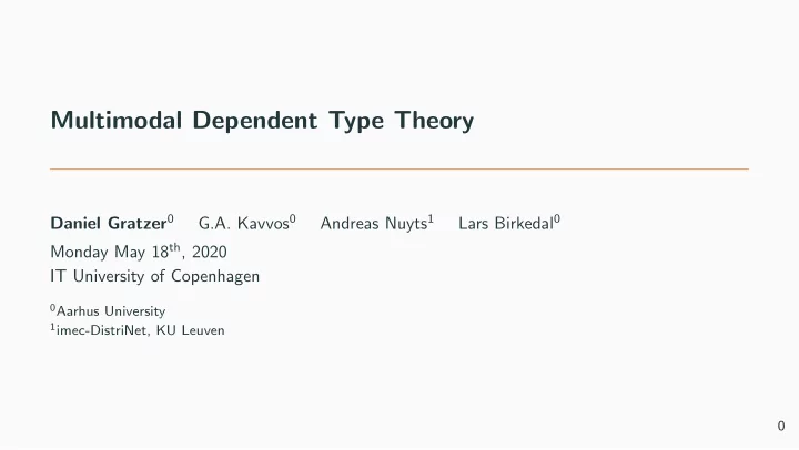
Multimodal Dependent Type Theory

Daniel Gratzer0 G.A. Kavvos0 Andreas Nuyts1 Lars Birkedal0 Monday May 18th, 2020 IT University of Copenhagen

0Aarhus University 1imec-DistriNet, KU Leuven

The problem

We’d like extend Martin-L¨

• f Type Theory and apply it to new situations.
• Staged programming [PD01].
• Proof-irrelevance [Pfe01].
• Guarded recursion [Clo+15; BGM17; Gua18].
• Parametric quantification [ND18].
• Exotic models of computation [Bir00].
• (Abstract) topology [Shu18].
• Differential geometry [Wel18].

1

Where do modalities come in?

Martin-L¨

• f Type Theory satisfies several desirable properties which help make it

convenient to use (canonicity, decidability of type-checking, etc.). Problem If we naively add new features, we will disrupt these properties. Solution Modalities can manage new features in a controlled way. Each example uses modalities to extended MLTT while preserving crucial properties.

2

A tangent: what exactly is a modality?

In general, people use modality to mean many different things:

• 1. Any unary type constructor.
• 2. A unary type constructor which is an internal functor.
• 3. A unary type constructor equipped with a monad structure.

For us, a modality is essentially a right adjoint.1 This restriction yields a practical syntax and still includes many examples.

1More specifically, a modality is essentially a dependent right adjoint [Bir+20]

3

A story of several type theories

Let us consider a representative example of how modal type theories are developed.

• 1. Work on guarded recursion converges towards the Fitch-style [BGM17; Clo18].
• 2. Birkedal et al. [Bir+20] isolate this into paradigmatic type theory.
• 3. Gratzer, Sterling, and Birkedal [GSB19] prove normalization for a similar system.

Each of these type theories build upon each other... but no reuse is possible.

4

Our Contribution: MTT

We introduce MTT: a type theory parameterized by a collection of modalities.

• MTT features usual connectives of Martin-L¨
• f Type Theory, including a universe.
• The user can instantiate MTT with different collections of modalities.
• Important results such as canonicity are proven irrespective of the modalities.

We have applied MTT to several different situations:

• Axiomatic cohesion
• Degrees of relatedness
• Guarded recursion and warps
• Various classic modal type theories

5

Revisiting our story

Let us reconsider the previous example with [Bir+20] and [GSB19]. With MTT we would not design two separate type theories!

• Instantiate MTT twice to yield type theories similar to the originals.
• Prove normalization for MTT once, and transfer the result to both instantiations.

MTT makes the superficial similarity into a formal relationship.

6

Modes and Mode theories

MTT is a multimode type theory, not just multimodal.

• Each mode is its own separate type theory, with modalities bridging between them.
• As an example, spatial type theory has two modes: sets and spaces.

7

Modes and Mode theories

MTT is a multimode type theory, not just multimodal.

• Each mode is its own separate type theory, with modalities bridging between them.
• As an example, spatial type theory has two modes: sets and spaces.

We follow [LS16; LSR17] and specify our modalities as a mode theory, a 2-category:

• bject ∼ mode

morphism ∼ modality 2-cell ∼ natural map between modalities

7

An example: an idempotent comonad

The mode theory for an idempotent comonad is generated from the following data:

• bjects: {m}

morphisms: {µ : m → m} 2-cells: {ǫ : µ ⇒ 1} Furthermore, µ ◦ µ = µ and that α = β for any pair of 2-cells.

8

An example: an idempotent comonad

The mode theory for an idempotent comonad is generated from the following data:

• bjects: {m}

morphisms: {µ : m → m} 2-cells: {ǫ : µ ⇒ 1} Furthermore, µ ◦ µ = µ and that α = β for any pair of 2-cells. This induces a single modality µ | − with the following operations: Γ ⊢ M : µ | A @ m Γ ⊢ extract(M) : A @ m Γ ⊢ M : µ | A @ m Γ ⊢ duplicate(M) : µ | µ | A @ m

8

An example: an idempotent comonad

The mode theory for an idempotent comonad is generated from the following data:

• bjects: {m}

morphisms: {µ : m → m} 2-cells: {ǫ : µ ⇒ 1} Furthermore, µ ◦ µ = µ and that α = β for any pair of 2-cells. This induces a single modality µ | − with the following operations: Γ ⊢ M : µ | A @ m Γ ⊢ extract(M) : A @ m Γ ⊢ M : µ | A @ m Γ ⊢ duplicate(M) : µ | µ | A @ m A mode annotation.

8

An example: an idempotent comonad

The mode theory for an idempotent comonad is generated from the following data:

• bjects: {m}

morphisms: {µ : m → m} 2-cells: {ǫ : µ ⇒ 1} Furthermore, µ ◦ µ = µ and that α = β for any pair of 2-cells. This induces a single modality µ | − with the following operations: Γ ⊢ M : µ | A @ m Γ ⊢ extract(M) : A @ m Γ ⊢ M : µ | A @ m Γ ⊢ duplicate(M) : µ | µ | A @ m A mode annotation. The fact that this mode theory is poset-enriched ensures that the comonad laws hold.

8

MTT, more formally

We will now introduce MTT a bit more carefully. Let us fix a mode theory M. MTT is stratified into the following judgments: Γ ctx @ m Γ ⊢ A type @ m Γ ⊢ M : A @ m Γ ⊢ δ : ∆ @ m Each judgment is localized to a mode and each mode contains a copy of MLTT.

9

MTT, more formally

We will now introduce MTT a bit more carefully. Let us fix a mode theory M. MTT is stratified into the following judgments: Γ ctx @ m Γ ⊢ A type @ m Γ ⊢ M : A @ m Γ ⊢ δ : ∆ @ m Each judgment is localized to a mode and each mode contains a copy of MLTT. We will ignore these today.

9

Modal types

Slogan: modalities act like functors between modes. Given a closed type A @ n and µ : n → m, there is a closed type µ | A @ m. This doesn’t easily scale to open types: Γ ⊢ A type @ n µ : n → m Γ ⊢ µ | A type @ m

10

Modal types

Slogan: modalities act like functors between modes. Given a closed type A @ n and µ : n → m, there is a closed type µ | A @ m. This doesn’t easily scale to open types: Γ ⊢ A type @ n µ : n → m Γ ⊢ µ | A type @ m One of these must live in the wrong mode.

10

Modal types

Slogan: modalities act like functors between modes. Given a closed type A @ n and µ : n → m, there is a closed type µ | A @ m. This doesn’t easily scale to open types: Γ ⊢ A type @ n µ : n → m Γ ⊢ µ | A type @ m One of these must live in the wrong mode. We require additional judgmental structure to make sense of modal types.

10

Fitch-style contexts

MTT uses a Fitch-style context so modalities to have an adjoint action on contexts: µ : n → m Γ ctx @ m Γ, µ ctx @ n While it is not entirely accurate, it is helpful to imagine −, µ ⊣ µ | −.

11

Fitch-style contexts

MTT uses a Fitch-style context so modalities to have an adjoint action on contexts: µ : n → m Γ ctx @ m Γ, µ ctx @ n While it is not entirely accurate, it is helpful to imagine −, µ ⊣ µ | −. Accordingly, the introduction and formation rules are transposition: µ : n → m Γ, µ ⊢ A type @ n Γ ⊢ µ | A type @ m µ : n → m Γ, µ ⊢ M : A @ n Γ ⊢ modµ(M) : µ | A @ m These rules follow other Fitch-style type theories [BGM17; Clo18; Bir+20; GSB19].

11

Fitch-style contexts with multiple modalities

Prior work had one modality, hence one lock. How do we scale to many modalities? Γ ctx @ m Γ = Γ, 1 ctx @ m ν : o → n µ : n → m Γ ctx @ m Γ, µ, ν = Γ, µ◦ν ctx @ o

12

Fitch-style contexts with multiple modalities

Prior work had one modality, hence one lock. How do we scale to many modalities? Γ ctx @ m Γ = Γ, 1 ctx @ m ν : o → n µ : n → m Γ ctx @ m Γ, µ, ν = Γ, µ◦ν ctx @ o In fact, is part of a 2-functor from Mcoop to contexts and substitutions. Definition Given a 2-cell α : µ ⇒ ν and a term Γ.ν ⊢ M : A @ m, there is a derived operation (−)α such that Γ.µ ⊢ Mα : Aα @ m. Secretly, this is built from a modal substitution behaving like a natural transformation.

12

What about variables?

Locks allow us to state the formation rule for modalities, but what about variables? With the standard variable rule, we again have a mode error! µ : n → m x : A, µ ⊢ x : A @ n

13

What about variables?

Locks allow us to state the formation rule for modalities, but what about variables? With the standard variable rule, we again have a mode error! µ : n → m x : A, µ ⊢ x : A @ n A must live in mode m A must live in mode n

13

What about variables?

Locks allow us to state the formation rule for modalities, but what about variables? With the standard variable rule, we again have a mode error! µ : n → m x : A, µ ⊢ x : A @ n

• Previous Fitch-style type theories handled this through an elimination rule.
• In MTT, we will introduce a final piece of judgmental structure.

13

Variable annotations

In addition to locks, each variable in the context will be annotated with a modality. µ : n → m Γ ctx @ m Γ, µ ⊢ A type @ n Γ, x : (µ | A) ctx @ m Another rough intuition: Γ, x : (µ | A) ∼ = Γ, x : µ | A.

14

Variable annotations

In addition to locks, each variable in the context will be annotated with a modality. µ : n → m Γ ctx @ m Γ, µ ⊢ A type @ n Γ, x : (µ | A) ctx @ m Another rough intuition: Γ, x : (µ | A) ∼ = Γ, x : µ | A. We can use these annotations to give a more sensible variable rule: µ : n → m Γ, x : (µ | A), µ ⊢ x : A @ n Intuition: this is the counit of the adjunction −, µ ⊣ µ | −.

14

What about 2-cells?

This variable rule is a bit restrictive; it requires the annotation and lock to match. We can relax a bit and require only a 2-cell between the annotation and the lock. µ, ν : n → m α : µ ⇒ ν Γ, x : (µ | A), ν ⊢ xα : Aα @ n In fact, this rule is a combination of the ‘counit’ rule and the action of on 2-cells.

15

Modal induction

The final piece of the puzzle is the elimination rule for µ | A.

• At a high-level this rule let’s us replace x : µ | A with y : (µ | A).
• We must generalize to replacing x : (ν | µ | A) with y : (ν ◦ µ | A).
• We rephrase this as a pattern-matching or cut-style rule.

16

Modal induction

The final piece of the puzzle is the elimination rule for µ | A.

• At a high-level this rule let’s us replace x : µ | A with y : (µ | A).
• We must generalize to replacing x : (ν | µ | A) with y : (ν ◦ µ | A).
• We rephrase this as a pattern-matching or cut-style rule.

Fix ν : m → o, µ : n → m. The elimination rule for µ is as follows: Γ, x : (ν | µ | A) ⊢ B type1 @ o Γ, y : (ν ◦ µ | A) ⊢ M1 : B[modµ(y)/x] @ o Γ, ν ⊢ M0 : µ | A @ m Γ ⊢ letν modµ(y) ← M0 in M1 : B[M0/x] @ o

16

Modal induction

The final piece of the puzzle is the elimination rule for µ | A.

• At a high-level this rule let’s us replace x : µ | A with y : (µ | A).
• We must generalize to replacing x : (ν | µ | A) with y : (ν ◦ µ | A).
• We rephrase this as a pattern-matching or cut-style rule.

Fix ν : m → o, µ : n → m. The elimination rule for µ is as follows: Γ, x : (ν | µ | A) ⊢ B type1 @ o Γ, y : (ν ◦ µ | A) ⊢ M1 : B[modµ(y)/x] @ o Γ, ν ⊢ M0 : µ | A @ m Γ ⊢ letν modµ(y) ← M0 in M1 : B[M0/x] @ o The motive

16

Modal induction

The final piece of the puzzle is the elimination rule for µ | A.

• At a high-level this rule let’s us replace x : µ | A with y : (µ | A).
• We must generalize to replacing x : (ν | µ | A) with y : (ν ◦ µ | A).
• We rephrase this as a pattern-matching or cut-style rule.

Fix ν : m → o, µ : n → m. The elimination rule for µ is as follows: Γ, x : (ν | µ | A) ⊢ B type1 @ o Γ, y : (ν ◦ µ | A) ⊢ M1 : B[modµ(y)/x] @ o Γ, ν ⊢ M0 : µ | A @ m Γ ⊢ letν modµ(y) ← M0 in M1 : B[M0/x] @ o The base case

16

Modal induction

The final piece of the puzzle is the elimination rule for µ | A.

• At a high-level this rule let’s us replace x : µ | A with y : (µ | A).
• We must generalize to replacing x : (ν | µ | A) with y : (ν ◦ µ | A).
• We rephrase this as a pattern-matching or cut-style rule.

Fix ν : m → o, µ : n → m. The elimination rule for µ is as follows: Γ, x : (ν | µ | A) ⊢ B type1 @ o Γ, y : (ν ◦ µ | A) ⊢ M1 : B[modµ(y)/x] @ o Γ, ν ⊢ M0 : µ | A @ m Γ ⊢ letν modµ(y) ← M0 in M1 : B[M0/x] @ o The term we pattern match on.

16

Taking stock of MTT

It’s easy to feel this is just “one damn rule after another”, but at a high-level: a modality for each morphism in M a coercion for each 2-cell in M modal introduction needs richer contexts we equip contexts with locks and make modalities ‘right adjoints’ we must factor locks into the variable rule we equip variables with modalities and occurences with 2-cells there is now a mismatch between modal annotations and types modal elimination moves from a modal type to an annotation

17

Summary of crucial modal rules

µ : n → m Γ ctx @ m Γ, µ ctx @ n µ : n → m Γ ctx @ m Γ, µ ⊢ A type1 @ n Γ, x : (µ | A) ctx @ m µ : n → m Γ, µ ⊢ A typeℓ @ n Γ ⊢ µ | A typeℓ @ m ν : m → n α : ν ⇒ locks(Γ1) Γ0, x : (ν | A), Γ1 ⊢ xα : Aα @ m µ : n → m Γ, µ ⊢ M : A @ n Γ ⊢ modµ(M) : µ | A @ m µ : n → m ν : m → o Γ, x : (ν | µ | A) ⊢ B type1 @ o Γ, ν ⊢ M0 : µ | A @ m Γ, x : (ν ◦ µ | A) ⊢ M1 : B[modµ(x)/x] @ o Γ ⊢ letν modµ(x) ← M0 in M1 : B[M0/x] @ o

18

Modal combinators

The mode theory is reflected into MTT as a series of modal combinators: 1 | A ≃ A µ | ν | A ≃ µ ◦ ν | A µ | A → ν | A (For each α : µ ⇒ ν) µ | A → B → (µ | A → µ | B) All of these follow because is a 2-functor out of Mcoop: Γ.1 = Γ ctx @ m Γ.µ.ν = Γ.µ◦ν ctx @ m Γ.ν ⊢ α

Γ : Γ.µ @ m 19

Example definitions of modal combinators

To get a feel for MTT, let us define some of these combinators. Programs coe[α : µ ⇒ ν](−) : µ | A → ν | Aα coe[α](x) Holes x : (1 | µ | A) ⊢ : ν | A

20

Example definitions of modal combinators

To get a feel for MTT, let us define some of these combinators. Programs coe[α : µ ⇒ ν](−) : µ | A → ν | Aα coe[α](x) let modµ(y) ← x in Holes x : (1 | µ | A), y : (µ | A) ⊢ : ν | A

20

Example definitions of modal combinators

To get a feel for MTT, let us define some of these combinators. Programs coe[α : µ ⇒ ν](−) : µ | A → ν | Aα coe[α](x) letν modµ(y) ← x in modν() Holes x : (1 | µ | A), x : (µ | A), ν ⊢ : A

20

Example definitions of modal combinators

To get a feel for MTT, let us define some of these combinators. Programs coe[α : µ ⇒ ν](−) : µ | A → ν | Aα coe[α](x) letν modµ(y) ← x in modν(yα) Holes

20

Example definitions of modal combinators

To get a feel for MTT, let us define some of these combinators. Programs coe[α : µ ⇒ ν](−) : µ | A → ν | Aα coe[α](x) letν modµ(y) ← x in modν(yα) compµ,ν(−) : µ ◦ ν | A → µ | ν | A comp(x) Holes x : (1 | µ ◦ ν | A) ⊢ : µ | ν | A

20

Example definitions of modal combinators

To get a feel for MTT, let us define some of these combinators. Programs coe[α : µ ⇒ ν](−) : µ | A → ν | Aα coe[α](x) letν modµ(y) ← x in modν(yα) compµ,ν(−) : µ ◦ ν | A → µ | ν | A comp(x) let modµ◦ν(y) ← x in Holes x : (· · · ), y : (µ ◦ ν | A) ⊢ : µ | ν | A

20

Example definitions of modal combinators

To get a feel for MTT, let us define some of these combinators. Programs coe[α : µ ⇒ ν](−) : µ | A → ν | Aα coe[α](x) letν modµ(y) ← x in modν(yα) compµ,ν(−) : µ ◦ ν | A → µ | ν | A comp(x) let modµ◦ν(y) ← x in modµ() Holes x : (· · · ), y : (µ ◦ ν | A), µ ⊢ : ν | A

20

Example definitions of modal combinators

To get a feel for MTT, let us define some of these combinators. Programs coe[α : µ ⇒ ν](−) : µ | A → ν | Aα coe[α](x) letν modµ(y) ← x in modν(yα) compµ,ν(−) : µ ◦ ν | A → µ | ν | A comp(x) let modµ◦ν(y) ← x in modµ(modν()) Holes x : (· · · ), y : (µ ◦ ν | A), µ◦ν ⊢ : A

20

Example definitions of modal combinators

To get a feel for MTT, let us define some of these combinators. Programs coe[α : µ ⇒ ν](−) : µ | A → ν | Aα coe[α](x) letν modµ(y) ← x in modν(yα) compµ,ν(−) : µ ◦ ν | A → µ | ν | A comp(x) let modµ◦ν(y) ← x in modµ(modν(y)) Holes

20

Results about MTT

A major strength of MTT is that we can prove theorems irrespective of M. Theorem (Consistency) There is no term · ⊢ M : IdB(tt, ff) @ m. Theorem (Canonicity) Subject to a technical restriction, if · ⊢ M : A @ m is a closed term, then the following conditions hold:

• If A = B, then · ⊢ M = tt : B @ m or · ⊢ M = ff : B @ m.
• If A = IdA0(N0, N1) then · ⊢ M = refl(N0) : IdA0(N0, N1) @ m.
• If A = µ | A0 then · ⊢ M = modµ(N) : µ | A0 @ m for some N.

As time permits we’ll return to canonicity, but for now just take it on faith.

21

Example: guarded recursion

The other major strength of MTT is that we can use it to model interesting examples!

• We’ll be interested in using MTT to model guarded recursion.
• Guarded recursion is naturally multimode.
• This situation crucially requires the interaction of modalities.

22

Guarded recursion: a brief introduction

Guarded recursion uses two modalities to isolate productive and coinductive programs.

23

Guarded recursion: a brief introduction

Guarded recursion uses two modalities to isolate productive and coinductive programs.

• 1. The later modality tags computation which are available at the next step:

next : A → A l¨

• b : (A → A) → A
• 2. The always modality tags computation which do not depend on the time step:

extract : A → A dup : A ≃ A These two modalities interact in a crucial way to give coinductive programs: now : A → A

23

Splitting guarded recursion into 2 modes

Previous guarded type theories had a single mode, we opt for 2 modes. t s

24

Splitting guarded recursion into 2 modes

Previous guarded type theories had a single mode, we opt for 2 modes. t s Varies with time (PSh(ω)). No notion of time (Set).

24

Splitting guarded recursion into 2 modes

Previous guarded type theories had a single mode, we opt for 2 modes. t s δ γ

24

Splitting guarded recursion into 2 modes

Previous guarded type theories had a single mode, we opt for 2 modes. t s δ Allow a constant type to trivially vary over time. γ

24

Splitting guarded recursion into 2 modes

Previous guarded type theories had a single mode, we opt for 2 modes. t s δ γ Restrict a varying type to global elements.

24

Splitting guarded recursion into 2 modes

Previous guarded type theories had a single mode, we opt for 2 modes. t s δ γ A δ ◦ γ | A

24

Splitting guarded recursion into 2 modes

Previous guarded type theories had a single mode, we opt for 2 modes. t s δ γ A δ ◦ γ | A ℓ A ℓ | A ΓA γ | A ∆A δ | A

24

Splitting guarded recursion into 2 modes

Previous guarded type theories had a single mode, we opt for 2 modes. t s δ γ A δ ◦ γ | A ℓ A ℓ | A ΓA γ | A ∆A δ | A δ ◦ γ ≤ 1 1 = γ ◦ δ 1 ≤ ℓ γ = γ ◦ ℓ

24

Modal operations

The terms for the following operations are all induced by generic combinators: next : A → A − ⊛− : (A → B) → A → B extract : A → A dup : A ≃ A now : A → A In particular, next and extract are instances of coercions, while dup and now follow from associativity.

25

What about L¨

• b?
• We can use the standard operations on MTT to derive all operations except L¨
• b.
• L¨
• b is actually a bit of problem; it’s a modality-specific operation!

26

What about L¨

• b?
• We can use the standard operations on MTT to derive all operations except L¨
• b.
• L¨
• b is actually a bit of problem; it’s a modality-specific operation!

Instead, we have to simply axiomitize L¨

• b:

Γ, x : (ℓ | A1≤ℓ) ⊢ M : A @ t Γ ⊢ l¨

• b(x. M) : A @ t

Γ, x : (ℓ | A1≤ℓ) ⊢ M : A @ t Γ ⊢ l¨

• b(x. M) = let modℓ(x) ← next(l¨
• b(x. M)) in M : A @ t

(NB: A1≤ℓ moves A from the Γ to Γ.ℓ)

26

What about L¨

• b?
• We can use the standard operations on MTT to derive all operations except L¨
• b.
• L¨
• b is actually a bit of problem; it’s a modality-specific operation!

Instead, we have to simply axiomitize L¨

• b:

Γ, x : (ℓ | A1≤ℓ) ⊢ M : A @ t Γ ⊢ l¨

• b(x. M) : A @ t

Γ, x : (ℓ | A1≤ℓ) ⊢ M : A @ t Γ ⊢ l¨

• b(x. M) = let modℓ(x) ← next(l¨
• b(x. M)) in M : A @ t

(NB: A1≤ℓ moves A from the Γ to Γ.ℓ) (NB: We follow Bizjak et al. [Biz+16] and just work in an extensional type theory.)

26

An aside: modality-specific operations

It’s not clear yet what the proper formulation of L¨

• b would be.

It belongs to a large class of operations which entangle a modality and another connective (in this case, → and ) which we term modality-specific. Question Is there a reasonable class of modality-specific operations that can be handled uniformly?

27

Programming in Guarded MTT

Now that we have these combinators established, we can use them to write guarded programs. Str′

A

l¨

• b(S. ∆(A) × S)

Str : U → U @ s Str(A) Γ(Str′

A) 28

Programming in Guarded MTT

Now that we have these combinators established, we can use them to write guarded programs. Str′

A

l¨

• b(S. ∆(A) × S)

Str : U → U @ s Str(A) Γ(Str′

A)

We only have one clock so coinductive streams only work on constant data.

28

Programming in Guarded MTT: zipWith

Now that streams are defined, we can write down an operator on them: go : ∆(A → B → C) → Str′

A → Str′ B → Str′ C

go(f ) l¨

• b(r. λx, y. (f ⊛δ xh ⊛δ yh, modℓ(r) ⊛ℓ xt ⊛ℓ yt))

29

Programming in Guarded MTT: zipWith

Now that streams are defined, we can write down an operator on them: go : ∆(A → B → C) → Str′

A → Str′ B → Str′ C

go(f ) l¨

• b(r. λx, y. (f ⊛δ xh ⊛δ yh, modℓ(r) ⊛ℓ xt ⊛ℓ yt))

zipWith : (A → B → C) → Str(A) → Str(B) → Str(C) zipWith(f )

• λx, y. modγ(go(modδ(f ))) ⊛γ x ⊛γ y

29

Programming in Guarded MTT: zipWith

Now that streams are defined, we can write down an operator on them: go : ∆(A → B → C) → Str′

A → Str′ B → Str′ C

go(f ) l¨

• b(r. λx, y. (f ⊛δ xh ⊛δ yh, modℓ(r) ⊛ℓ xt ⊛ℓ yt))

zipWith : (A → B → C) → Str(A) → Str(B) → Str(C) zipWith(f )

• λx, y. modγ(go(modδ(f ))) ⊛γ x ⊛γ y

We can use the ambient dependent type theory to show that zipWith preserves e.g. commutativity.

29

Guarded recursion conclusions

Experimentally, this calculus for guarded recursion is reasonably pleasant for pen-and-paper calculations! There are a few missing things:

• 1. Using extensional type theory makes a standard implementation impossible.
• 2. Using only and makes a few things simple, but lacks the expressivity of

clocks. Going forward, we’d like to address these limitations, especially the first!

30

Conclusions

We introduce MTT: a type theory parameterized by a collection of modalities.

• MTT features usual connectives of Martin-L¨
• f Type Theory, including a universe.
• The user can instantiate MTT with different collections of modalities.
• Important results such as canonicity are proven irrespective of the modalities.

We have applied MTT to several different situations:

• Axiomatic cohesion
• Degrees of relatedness
• Guarded recursion and warps
• Various classic modal type theories

https://jozefg.github.io/papers/multimodal-dependent-type-theory.pdf https://jozefg.github.io/papers/type-theory-a-la-mode.pdf

31

Bonus slides!

Bonus slides is code for “very technical slides I liked too much to delete entirely”.

32

The modal substitution calculus

Before we talk about the canonicity proof, we need to quickly show the explicit substitution calculus. µ : n → m Γ ⊢ δ : ∆ @ m Γ.µ ⊢ δ.µ : ∆.µ @ n α : µ ⇒ ν Γ.ν ⊢ α

Γ : Γ.µ @ n

Γ ⊢ δ : ∆ @ m Γ ⊢ δ.1 = δ : ∆ @ m µ : n → m ν : o → n Γ ⊢ δ : ∆ @ m Γ.µ◦ν ⊢ δ.µ◦ν = δ.µ.ν : ∆.µ◦ν @ m µ, ν : n → m α : ν ⇒ µ Γ ⊢ δ : ∆ @ m Γ.µ ⊢ α

∆ ◦ (δ.µ) = (δ.ν) ◦ α Γ : ∆.ν @ n 33

Proving canonicity via gluing proof

How does gluing work?

• 1. Define a category of models, syntax is (by definition) the initial model.
• 2. Define G which equips elements of some model M with a proof of e.g. canonicity.
• 3. Define a projection from the M to the G which forgets the proof.
• 4. Use the initiality of syntax to obtain a section to projection.
• 5. Conclude that every element of the initial model enjoys e.g. canonicity.

Best thought of as a categorification of logical relations, where we also allow proof relevance.

34

Advantage of the gluing approach

• We can already attempt to prove e.g. canonicity via standard syntactic logical

relations.

• The goal is to make these proofs simpler by excavating the categorical structure.
• Another big advantage is the switch to proof-relevance: necessary to handle

universes well!

35

Where do I learn more?

Gluing is not a new idea, but two recent preprints cover some of my own perspectives

• n it:
• 1. Sterling and Spitters [SS18], an arxiv preprint about the simply-typed case.
• 2. Sterling, Angiuli, and Gratzer [SAG20], another preprint covering the

dependently-typed case. The key line of development at the moment is how to make gluing more mathematical. Frustratingly, the ideas proposed in the latter are complex to scale to modalities.

36

The models of MTT

In order to apply gluing, we construct a category of models for MTT [Car78].

• A model of MTT is built around a 2-functor M : M → Cat which sends each

mode to a category of contexts.

• We require a CWF for each M[m] (including ,,Id,etc.).
• Each 1-cell in M must induce a modality relating the two different modes.

NB: If we instead worked with dependent right adjoints, this becomes even simpler because a modality has such a nice semantic characterization!

37

The technical restriction

The difficulty in the gluing proof for MTT is handling modalities in the glued model.

• 1. I know how to do this in a very clean way for simply-typed languages or when the

modalities are dependent right adjoints, but it’s hard in MTT.

• 2. In order to simplify, we insist ·.µ = · (the left adjoint preserves terminals).
• 3. We are presently working to remove this restriction.

Why does this restriction help? It allows us to work exclusively with closed terms. Otherwise we need to also work with terms in the context ·.µ. Further details for our proof are given in the accompanying technical report.

38