Multidimensional Scaling MAT 6480W / STT 6705V Guy Wolf - PowerPoint PPT Presentation
Geometric Data Analysis Multidimensional Scaling MAT 6480W / STT 6705V Guy Wolf guy.wolf@umontreal.ca Universit e de Montr eal Fall 2019 MAT 6480W (Guy Wolf) MDS UdeM - Fall 2019 1 / 29 Outline Multidimensional scaling (MDS) 1
Geometric Data Analysis Multidimensional Scaling MAT 6480W / STT 6705V Guy Wolf guy.wolf@umontreal.ca Universit´ e de Montr´ eal Fall 2019 MAT 6480W (Guy Wolf) MDS UdeM - Fall 2019 1 / 29
Outline Multidimensional scaling (MDS) 1 Gram matrix Double-centering Stress function Distance metrics 2 Minkowski distances Mahalanobis distance Hamming distance Similarities and dissimilarities 3 Gaussian affinities Cosine similarities Jaccard index Dynamic time-warp 4 Comparing misaligned signals Computing DTW dissimilarity Combining similarities 5 MAT 6480W (Guy Wolf) MDS UdeM - Fall 2019 2 / 29
Multidimensional scaling What if we cannot compute a covariance matrix? Consider a k -dimensional rigid body - all we need to know are distances between its parts. We can ignore its position and orientation and find the most “efficient” way to place it in ❘ k . MAT 6480W (Guy Wolf) MDS UdeM - Fall 2019 3 / 29
Multidimensional scaling 0 · · · d 1 j · · · d 1 m . . ... . . . . � y 1 , . . . , y m ∈ ❘ k : � D = 0 �→ d i 1 d im � y i − y j � = d ij = � x i − x j � . . ... . . . . d m 1 · · · d mj · 0 Multidimensional scaling Given a m × m matrix D of distances between m objects, find k dimensional coordinates that preserve these distances. MAT 6480W (Guy Wolf) MDS UdeM - Fall 2019 3 / 29
Multidimensional scaling Gram matrix A distance matrix is not convenient to directly embed in ❘ k , but embedding inner products is a simpler task. Gram matrix A matrix G that contains inner products g ij = � x i , x j � is a Gram matrix. Using the spectral theorem we can decompose G = ΦΛΦ T and get m � λ q Φ[ i , q ]Φ[ j , q ] = � Φ[ i , · ]Λ 1 / 2 , Φ[ j , · ]Λ 1 / 2 � � x i , x j � = g ij = q =1 Similar to PCA, we can truncate small eigenvalues and use the k biggest eigenpairs. MAT 6480W (Guy Wolf) MDS UdeM - Fall 2019 4 / 29
Multidimensional scaling Spectral embedding � G � = λ 1 ≥ ≥ λ 3 ≥ · · · ≥ λ k > 0 λ 2 m φ 1 φ 2 φ 3 · · · φ k MAT 6480W (Guy Wolf) MDS UdeM - Fall 2019 5 / 29
Multidimensional scaling Spectral embedding � G � = λ 1 ≥ ≥ λ 3 ≥ · · · ≥ λ k > 0 λ 2 m φ 1 φ 2 φ 3 · · · φ k MAT 6480W (Guy Wolf) MDS UdeM - Fall 2019 5 / 29
Multidimensional scaling Spectral embedding � G � = λ 1 ≥ ≥ λ 3 ≥ · · · ≥ λ k > 0 λ 2 m φ 1 φ 2 φ 3 · · · φ k x �→ Φ( x ) � [ λ 1 / 2 1 φ 1 ( x ) , λ 1 / 2 2 φ 2 ( x ) , λ 1 / 2 3 φ 3 ( x ) , . . . , λ 1 / 2 k φ k ( x )] T MAT 6480W (Guy Wolf) MDS UdeM - Fall 2019 5 / 29
Multidimensional scaling Double-centering Notice that given a distance metric that is equivalent to Euclidean distances, we can write: � x − y � 2 = � x � 2 + � y � 2 − 2 � x , y � But then: MAT 6480W (Guy Wolf) MDS UdeM - Fall 2019 6 / 29
Multidimensional scaling Double-centering Notice that given a distance metric that is equivalent to Euclidean distances, we can write: � x − y � 2 = � x � 2 + � y � 2 − 2 � x , y � But then: mean x ( � x − y � 2 ) = � z � 2 + � y � 2 − 2 � z , y � where z and � z � 2 are the mean and mean squared norm of the data MAT 6480W (Guy Wolf) MDS UdeM - Fall 2019 6 / 29
Multidimensional scaling Double-centering Notice that given a distance metric that is equivalent to Euclidean distances, we can write: � x − y � 2 = � x � 2 + � y � 2 − 2 � x , y � But then: mean x ( � x − y � 2 ) = � z � 2 + � y � 2 − 2 � z , y � mean y ( � x − y � 2 ) = � z � 2 + � x � 2 − 2 � x , z � where z and � z � 2 are the mean and mean squared norm of the data MAT 6480W (Guy Wolf) MDS UdeM - Fall 2019 6 / 29
Multidimensional scaling Double-centering Notice that given a distance metric that is equivalent to Euclidean distances, we can write: � x − y � 2 = � x � 2 + � y � 2 − 2 � x , y � But then: mean x ( � x − y � 2 ) = � z � 2 + � y � 2 − 2 � z , y � mean y ( � x − y � 2 ) = � z � 2 + � x � 2 − 2 � x , z � mean x , y ( � x − y � 2 ) = 2 � z � 2 − 2 � z , z � where z and � z � 2 are the mean and mean squared norm of the data MAT 6480W (Guy Wolf) MDS UdeM - Fall 2019 6 / 29
Multidimensional scaling Double-centering Thus, if we set g ( x , y ) = − 2 − 1 � � x − y � 2 − mean x ( � x − y � 2 ) � − mean y ( � x − y � 2 ) + mean x , y ( � x − y � 2 ) we get a gram matrix, since: g ( x , y ) = ( � x , y � − � x , z � ) − ( � z , y � − � z , z � ) = � x − z , y − z � � �� � � �� � � x , y − z � � z , y − z � 2 J D (2) J where J = Id − 1 m � 1 � Therefore, we can compute G = − 1 1 T MAT 6480W (Guy Wolf) MDS UdeM - Fall 2019 6 / 29
Multidimensional scaling Classic MDS Classic MDS is computed with the following algorithm: MDS algorithm Formulate squared distances 1 Build Gram matrix by double-centering 2 SVD (or eigendecomposition) 3 Assign coordinates based on eigenvalues and eigenvectors 4 Exercise: show that for centered data in Euclidean space this embedding is identical to PCA. MAT 6480W (Guy Wolf) MDS UdeM - Fall 2019 7 / 29
Multidimensional scaling Stress function What if we are not given a distance metric, but just dissimilarities? Stress function A function that quantifies the disagreement between given dissimilarities and embedded Euclidean distances. Examples Stress functions � i < j (ˆ d ij − f ( d ij )) 2 Metric MDS stress: , where f is a predetermined � i < j d 2 ij monotonically increasing function � i < j (ˆ d ij − f ( d ij )) 2 Kruskal’s stress-1: , where f is optimized, but still � i < j ˆ d 2 ij monotonically increasing (ˆ d ij − d ij ) 2 Sammon’s stress: ( � i < j d ij ) − 1 � i < j d ij MAT 6480W (Guy Wolf) MDS UdeM - Fall 2019 8 / 29
Multidimensional scaling Non-metric MDS Non-metric, or non-classical MDS is computed by the following algorithm: Non-metric MDS algorithm Formulate a dissimilarity matrix D . 1 Find an initial configuration (e.g., using classical MDS) with 2 distance matrix ˆ D . Minimize STRESS D ( f , ˆ D ) by optimizing the fitting function. 3 Minimize STRESS D ( f , ˆ D ) by optimizing the configuration and 4 resulting ˆ D . Iterate the previous two steps until the stress is lower than a 5 stopping threshold. MAT 6480W (Guy Wolf) MDS UdeM - Fall 2019 9 / 29
Distance metrics Metric spaces Consider a dataset X as an arbitrary collection of data points Distance metric A distance metric is a function d : X × X → [0 , ∞ ) that satisfies three conditions for any x , y , z ∈ X : d ( x , y ) = 0 ⇔ x = y 1 d ( x , y ) = d ( y , x ) 2 d ( x , y ) ≤ d ( x , z ) + d ( z , y ) 3 The set X of data points together with an appropriate distance metric d ( · , · ) is called a metric space. MAT 6480W (Guy Wolf) MDS UdeM - Fall 2019 10 / 29
Distance metrics Euclidean distance When X ⊂ ❘ n we can consider Euclidean distances: Euclidean distance The distance between x , y ∈ X is defined by � x − y � 2 = � n i =1 ( x [ i ] − y [ i ]) 2 One of the classic most common distance metrics Often inappropriate in realistic settings without proper preprocessing & feature extraction Also used for least mean square error optimizations Proximity requires all attributes to have equally small differences MAT 6480W (Guy Wolf) MDS UdeM - Fall 2019 11 / 29
Distance metrics Manhattan distances Manhattan distance The Manhattan distance between x , y ∈ X is defined by � x − y � 1 = � n i =1 | x [ i ] − y [ i ] | . This distance is also called taxicab or cityblock distance Taken from Wikipedia MAT 6480W (Guy Wolf) MDS UdeM - Fall 2019 12 / 29
Distance metrics Minkowski ( ℓ p ) distance Minkowski distance The Minkowski distance between x , y ∈ X ⊂ ❘ n is defined by n � � x − y � p | x [ i ] − y [ i ] | p p = i =1 for some p > 0. This is also called the ℓ p distance. Three popular Minkowski distances are: Manhattan distance: � x − y � 1 = � n p = 1 i =1 | x [ i ] − y [ i ] | i =1 | x [ i ] − y [ i ] | 2 � n p = 2 Euclidean distance: � x − y � 2 = p = ∞ Supremum/ ℓ max distance: � x − y � ∞ = sup 1 ≤ i ≤ n | x [ i ] − y [ i ] | MAT 6480W (Guy Wolf) MDS UdeM - Fall 2019 13 / 29
Distance metrics Normalization & standardization Minkowski distances require normalization to deal with varying magnitudes, scaling, distribution or measurement units. Min-max normalization minmax( x )[ i ] = x [ i ] − m i , where m i and r i are the min value and range r i of attribute i . Z-score standardization zscore( x )[ i ] = x [ i ] − µ i , where µ i and σ i are the mean and STD of σ i attribute i . log attenuation logatt( x )[ i ] = sgn( x [ i ]) log( | x [ i ] | + 1) MAT 6480W (Guy Wolf) MDS UdeM - Fall 2019 14 / 29
Recommend
More recommend
Explore More Topics
Stay informed with curated content and fresh updates.

