Multi-join Query Evaluation on Big Data Lecture 3 Dan Suciu March, - PowerPoint PPT Presentation
Algorithm Lower Bound Equivalence Summary Multi-join Query Evaluation on Big Data Lecture 3 Dan Suciu March, 2015 Dan Suciu Multi-Joins Lecture 3 March, 2015 1 / 26 Algorithm Lower Bound Equivalence Summary Multi-join Query
Algorithm Lower Bound Equivalence Summary Multi-join Query Evaluation on Big Data Lecture 3 Dan Suciu March, 2015 Dan Suciu Multi-Joins – Lecture 3 March, 2015 1 / 26
Algorithm Lower Bound Equivalence Summary Multi-join Query Evaluation – Outline Part 1 Optimal Sequential Algorithms. Part 2 Lower bounds for Parallel Algorithms. Part 3 Optimal Parallel Algorithms. Part 3 Data Skew. Dan Suciu Multi-Joins – Lecture 3 March, 2015 2 / 26
Algorithm Lower Bound Equivalence Summary Summary so far Q ( x ) = R 1 ( x 1 ) ,..., R ℓ ( x ℓ ) ∣ R 1 ∣ = m 1 ,..., ∣ R ℓ ∣ = m ℓ Sequential World Cost: output size of Q Upper bound AGM ( Q ) = m ρ ∗ . Fractional edge cover. Lower bound (tightness): fractional vertex packing Generic-join algorithm. Parallel World Cost: communication. 1-round, skew-free, equal-cardinalities. Lower bound m / p 1 / τ ∗ . Fractional edge packing Upper bound: fractional vertex cover. HyperCube algorithm. Dan Suciu Multi-Joins – Lecture 3 March, 2015 3 / 26
Algorithm Lower Bound Equivalence Summary Summary so far Q ( x ) = R 1 ( x 1 ) ,..., R ℓ ( x ℓ ) ∣ R 1 ∣ = m 1 ,..., ∣ R ℓ ∣ = m ℓ Sequential World Cost: output size of Q Upper bound AGM ( Q ) = m ρ ∗ . Fractional edge cover. Lower bound (tightness): fractional vertex packing Generic-join algorithm. Parallel World Cost: communication. 1-round, skew-free, equal-cardinalities. Lower bound m / p 1 / τ ∗ . Fractional edge packing Upper bound: fractional vertex cover. HyperCube algorithm. Dan Suciu Multi-Joins – Lecture 3 March, 2015 3 / 26
Algorithm Lower Bound Equivalence Summary Summary so far Q ( x ) = R 1 ( x 1 ) ,..., R ℓ ( x ℓ ) ∣ R 1 ∣ = m 1 ,..., ∣ R ℓ ∣ = m ℓ Sequential World Cost: output size of Q Upper bound AGM ( Q ) = m ρ ∗ . Fractional edge cover. Lower bound (tightness): fractional vertex packing Generic-join algorithm. Parallel World Cost: communication. 1-round, skew-free, equal-cardinalities. Lower bound m / p 1 / τ ∗ . Fractional edge packing Upper bound: fractional vertex cover. HyperCube algorithm. Dan Suciu Multi-Joins – Lecture 3 March, 2015 3 / 26
Algorithm Lower Bound Equivalence Summary Outline of Lecture 3 HyperCube Algorithm for arbitrary cardinalities Lower bound formula for arbitrary cardinalities Prove that they are equal Summary Will consider only databases without skew Dan Suciu Multi-Joins – Lecture 3 March, 2015 4 / 26
Algorithm Lower Bound Equivalence Summary Why Databases without Skew Matter In practice, skewed values are detected and treated separately; cost should be a function of the degree of skew. Example: join Q ( x , y , z ) = R ( x , y ) , S ( y , z ) . Without skew: L = m / p . (Common case) With skew, as bad as cartesian product: L ≥ m / p 1 / 2 . In general, for any query Q : Without skew: L = m / p 1 / τ ∗ . With skew: L ≥ m / p 1 / ρ ∗ (lecture 2) Dan Suciu Multi-Joins – Lecture 3 March, 2015 5 / 26
Algorithm Lower Bound Equivalence Summary Review of the HyperCube Algorithm Afrati and Ullman described in EDBT’2010 an algorithm for computing any conjunctive in one MapReduce job. Same as a one-round algorithm on the MPC model. Later, it was called the Shares algorithm. Beame, Koutris, and S. analyzed in PODS’2013 and PODS ’2014 the parameters for the algorithm, and called it the HyperCube algorithm. We will use this name. Dan Suciu Multi-Joins – Lecture 3 March, 2015 6 / 26
Algorithm Lower Bound Equivalence Summary Review of the HyperCube Algorithm Q ( x ) = R 1 ( x 1 ) ,..., R ℓ ( x ℓ ) ∣ R 1 ∣ = m 1 ,..., ∣ R ℓ ∣ = m ℓ Compute Q on p servers. Dan Suciu Multi-Joins – Lecture 3 March, 2015 7 / 26
Algorithm Lower Bound Equivalence Summary Review of the HyperCube Algorithm Q ( x ) = R 1 ( x 1 ) ,..., R ℓ ( x ℓ ) ∣ R 1 ∣ = m 1 ,..., ∣ R ℓ ∣ = m ℓ Compute Q on p servers. Organize the p servers in a hypercube: [ p ] = [ p 1 ] × ⋯ × [ p k ] . The numbers p 1 ,..., p k are called shares . Choose k independent hash functions h 1 ,..., h k Round 1 Each server sends each tuple R j ( x j 1 , x j 2 ,... ) to all servers whose coordinates j 1 , j 2 ,... are h j 1 ( x j 1 ) , h j 2 ( x j 2 ) ,... and broadcasts along the missing dimensions. Then, each server computes Q on its local data. Problem: compute the shares p 1 ,..., p k . Dan Suciu Multi-Joins – Lecture 3 March, 2015 7 / 26
Algorithm Lower Bound Equivalence Summary They HyperCube Algorithm – Computing the Shares Q ( x ) = R 1 ( x 1 ) ,..., R ℓ ( x ℓ ) ∣ R 1 ∣ = m 1 ,..., ∣ R ℓ ∣ = m ℓ The Shares-Problem Find shares p 1 ,..., p k s.t. ∏ i p i = p and the load is minimized. m j Number of tuples that a server receives from R j is: ∏ i ∈ Rj p i Dan Suciu Multi-Joins – Lecture 3 March, 2015 8 / 26
Algorithm Lower Bound Equivalence Summary They HyperCube Algorithm – Computing the Shares Q ( x ) = R 1 ( x 1 ) ,..., R ℓ ( x ℓ ) ∣ R 1 ∣ = m 1 ,..., ∣ R ℓ ∣ = m ℓ The Shares-Problem Find shares p 1 ,..., p k s.t. ∏ i p i = p and the load is minimized. m j Number of tuples that a server receives from R j is: ∏ i ∈ Rj p i [Afrati&Ullman’10] Optimize L = ∑ j m j ∏ i ∈ Rj p i . Non-linear. Dan Suciu Multi-Joins – Lecture 3 March, 2015 8 / 26
Algorithm Lower Bound Equivalence Summary They HyperCube Algorithm – Computing the Shares Q ( x ) = R 1 ( x 1 ) ,..., R ℓ ( x ℓ ) ∣ R 1 ∣ = m 1 ,..., ∣ R ℓ ∣ = m ℓ The Shares-Problem Find shares p 1 ,..., p k s.t. ∏ i p i = p and the load is minimized. m j Number of tuples that a server receives from R j is: ∏ i ∈ Rj p i [Afrati&Ullman’10] Optimize L = ∑ j m j ∏ i ∈ Rj p i . Non-linear. m j [Beame’14] Optimize L = max j ∏ i ∈ Rj p i : minimize L p 1 ⋅ p 2 ⋯ p k ≤ p The Shares Problem: m j ∀ j ∶ L ≥ ∏ i ∈ Rj p i Will show that this is equivalent to a linear optimization problem. Dan Suciu Multi-Joins – Lecture 3 March, 2015 8 / 26
Algorithm Lower Bound Equivalence Summary E-Shares: A Linear Optimization Problem Q ( x ) = R 1 ( x 1 ) ,..., R ℓ ( x ℓ ) ∣ R 1 ∣ = m 1 ,..., ∣ R ℓ ∣ = m ℓ Optimization problem: find shares p 1 ,..., p ℓ such that The Shares Problem The E-Shares Linear Problem Parameter: Value: Shares p 1 ,..., p k Sizes m 1 ,..., m ℓ Load L minimize L p 1 ⋅ p 2 ⋯ p k ≤ p Optimize: m j ∀ j ∶ L ≥ ∏ i ∈ Rj p i Dan Suciu Multi-Joins – Lecture 3 March, 2015 9 / 26
Algorithm Lower Bound Equivalence Summary E-Shares: A Linear Optimization Problem Q ( x ) = R 1 ( x 1 ) ,..., R ℓ ( x ℓ ) ∣ R 1 ∣ = m 1 ,..., ∣ R ℓ ∣ = m ℓ Optimization problem: find shares p 1 ,..., p ℓ such that The Shares Problem The E-Shares Linear Problem Parameter: Value: log p Value: Shares p 1 ,..., p k Sizes m 1 ,..., m ℓ Load L minimize L p 1 ⋅ p 2 ⋯ p k ≤ p Optimize: m j ∀ j ∶ L ≥ ∏ i ∈ Rj p i Dan Suciu Multi-Joins – Lecture 3 March, 2015 9 / 26
Algorithm Lower Bound Equivalence Summary E-Shares: A Linear Optimization Problem Q ( x ) = R 1 ( x 1 ) ,..., R ℓ ( x ℓ ) ∣ R 1 ∣ = m 1 ,..., ∣ R ℓ ∣ = m ℓ Optimization problem: find shares p 1 ,..., p ℓ such that The Shares Problem The E-Shares Linear Problem Parameter: Value: log p Value: Shares p 1 ,..., p k e 1 ,..., e k Sizes m 1 ,..., m ℓ µ 1 ,...,µ ℓ Load L λ minimize L p 1 ⋅ p 2 ⋯ p k ≤ p Optimize: m j ∀ j ∶ L ≥ ∏ i ∈ Rj p i Dan Suciu Multi-Joins – Lecture 3 March, 2015 9 / 26
Algorithm Lower Bound Equivalence Summary E-Shares: A Linear Optimization Problem Q ( x ) = R 1 ( x 1 ) ,..., R ℓ ( x ℓ ) ∣ R 1 ∣ = m 1 ,..., ∣ R ℓ ∣ = m ℓ Optimization problem: find shares p 1 ,..., p ℓ such that The Shares Problem The E-Shares Linear Problem Parameter: Value: log p Value: Shares p 1 ,..., p k e 1 ,..., e k Sizes m 1 ,..., m ℓ µ 1 ,...,µ ℓ Load L λ minimize L minimize λ p 1 ⋅ p 2 ⋯ p k ≤ p Optimize: − e 1 − e 2 − ... − e k ≥ − 1 λ + ∑ i ∶ i ∈ R j e i ≥ µ j m j ∀ j ∶ L ≥ ∀ j ∶ ∏ i ∈ Rj p i Dan Suciu Multi-Joins – Lecture 3 March, 2015 9 / 26
Algorithm Lower Bound Equivalence Summary E-Shares: A Linear Optimization Problem Q ( x ) = R 1 ( x 1 ) ,..., R ℓ ( x ℓ ) ∣ R 1 ∣ = m 1 ,..., ∣ R ℓ ∣ = m ℓ Optimization problem: find shares p 1 ,..., p ℓ such that The Shares Problem The E-Shares Linear Problem Parameter: Value: log p Value: Shares p 1 ,..., p k e 1 ,..., e k Sizes m 1 ,..., m ℓ µ 1 ,...,µ ℓ Load L λ minimize L minimize λ p 1 ⋅ p 2 ⋯ p k ≤ p Optimize: − e 1 − e 2 − ... − e k ≥ − 1 λ + ∑ i ∶ i ∈ R j e i ≥ µ j m j ∀ j ∶ L ≥ ∀ j ∶ ∏ i ∈ Rj p i Optimal shares: p 1 = p e ∗ 1 ,..., p k = p e ∗ Optimal load: L = p λ ∗ k Dan Suciu Multi-Joins – Lecture 3 March, 2015 9 / 26
Algorithm Lower Bound Equivalence Summary Discussion For equal-cardinalities, L = m / p 1 / τ ∗ . Speedup given by the optimal fractional edge packing. What is the speedup now? The E-Shares formula L = p λ ∗ is not insightful, as λ ∗ depends on µ 1 ,...,µ ℓ . Goal: analyze how L depends on p (speedup) and on the cardinalities m 1 ,..., m ℓ . Dan Suciu Multi-Joins – Lecture 3 March, 2015 10 / 26
Recommend
More recommend
Explore More Topics
Stay informed with curated content and fresh updates.
