Motion Tracking CS6240 Multimedia Analysis Leow Wee Kheng - PowerPoint PPT Presentation
Motion Tracking CS6240 Multimedia Analysis Leow Wee Kheng Department of Computer Science School of Computing National University of Singapore (CS6240) Motion Tracking 1 / 55 Introduction Introduction Video contains motion information
Motion Tracking CS6240 Multimedia Analysis Leow Wee Kheng Department of Computer Science School of Computing National University of Singapore (CS6240) Motion Tracking 1 / 55
Introduction Introduction Video contains motion information which can be used for detecting the presence of moving objects tracking and analyzing the motion of the objects tracking and analyzing the motion of camera Basic tracking methods: Gradient-based Image Flow: Track points based on intensity gradient. Example: Lucas-Kanade method [LK81, TK91]. Feature-based Image Flow: Track points based on template matching of features at points. Mean Shift Tracking: Track image patches based on feature distributions, e.g., color histograms [CRM00]. (CS6240) Motion Tracking 2 / 55
Introduction Strengths and Weaknesses Image flow approach: Very general and easy to use. If track correctly, can obtain precise trajectory with sub-pixel accuracy. Easily confused by points with similar features. Cannot handle occlusion. Cannot differentiate between planner motion and motion in depth. Demo: lk-elephant.mpg. Mean shift tracking: Very general and easy to use. Can track objects that change size & orientation. Can handle occlusion, size change. Track trajectory not as precise. Can’t track object boundaries accurately. Demo: ms-football1.avi, ms-football2.avi. (CS6240) Motion Tracking 3 / 55
Introduction Basic methods can be easily confused in complex situations: frame 1 frame 2 In frame 1, which hand is going which way? Which hand in frame 1 corresponds to which hand in frame 2? (CS6240) Motion Tracking 4 / 55
Introduction Notes: The chances of making wrong association is reduced if we can correctly predict where the objects will be in frame 2. To predict ahead of time, need to estimate the velocities and the positions of the objects in frame 1. To overcome these problems, need more sophisticated tracking algorithms: Kalman filtering: for linear dynamic systems, unimodal probability distributions Extended Kalman filtering: for nonlinear dynamic systems, unimodal probability distributions Condensation algorithm: for multi-modal probability distributions (CS6240) Motion Tracking 5 / 55
Kalman Filtering g - h Filter g - h Filter Consider 1-D case and suppose object travels at constant speed. Let x n and ˙ x n denote position and speed of object at time step n . Then, at time step n + 1, we have x n +1 = x n + ˙ x n T (1) x n +1 ˙ = x n ˙ (2) where T is the time interval between time steps. These equations are called the system dynamic model. Suppose at time step n , measured position y n � = estimated position x n . Then, update speed ˙ x n of object as follows: y n − x n x n ← ˙ ˙ x n + h n (3) T where h n is a small parameter. (CS6240) Motion Tracking 6 / 55
Kalman Filtering g - h Filter Notes: If x n < y n , then estimated speed < actual speed. Algorithm 3 increases the estimated speed. If x n > y n , then estimated speed > actual speed. Algorithm 3 decreases the estimated speed. After updating for several times, the estimated speed will become closer and closer to the actual speed. (CS6240) Motion Tracking 7 / 55
Kalman Filtering g - h Filter Another way of writing Algorithm 3 is as the following equation: y n − x ∗ n,n − 1 x ∗ x ∗ ˙ n,n = ˙ n,n − 1 + h n . (4) T x ∗ ˙ n,n − 1 = predicted estimate: the estimation of ˙ x at time step n based on past measurements made up to time step n − 1. x ∗ ˙ n,n = filtered estimate: the estimation of ˙ x at time step n based on past measurements made up to time step n . Some books use this notation: y n − x ∗ n | n − 1 x ∗ x ∗ ˙ n | n = ˙ n | n − 1 + h n . (5) T (CS6240) Motion Tracking 8 / 55
Kalman Filtering g - h Filter The estimated position can be updated in a similar way: x ∗ n,n = x ∗ n,n − 1 + g n ( y n − x ∗ n,n − 1 ) (6) where g n is a small parameter. Taken together, the two estimation equations form the g - h track update or filtering equations [Bro98]: n,n − 1 + h n x ∗ x ∗ T ( y n − x ∗ ˙ = ˙ n,n − 1 ) (7) n,n x ∗ x ∗ n,n − 1 + g n ( y n − x ∗ = n,n − 1 ) . (8) n,n (CS6240) Motion Tracking 9 / 55
Kalman Filtering g - h Filter Now, we can use the system dynamic equations to predict the object’s position and speed at time step n + 1. First, we rewrite the equations using the new notation to obtain the g - h state transition or prediction equations: x ∗ x ∗ ˙ = ˙ (9) n +1 ,n n,n x ∗ x ∗ x ∗ = n,n + ˙ n,n T (10) n +1 ,n x ∗ x ∗ = n,n + ˙ n +1 ,n T . (11) Substituting these equations into the filtering equations yield the g - h tracking-filter equations: n,n − 1 + h n x ∗ x ∗ T ( y n − x ∗ ˙ = ˙ n,n − 1 ) (12) n +1 ,n x ∗ x ∗ x ∗ n +1 ,n + g n ( y n − x ∗ = n,n − 1 + T ˙ n,n − 1 ) . (13) n +1 ,n (CS6240) Motion Tracking 10 / 55
Kalman Filtering g - h Filter These equations also describe many other filters, e.g., Wiener filter Kalman filter Bayes filter Least-squares filter etc... They differ in their choices of g n and h n . (CS6240) Motion Tracking 11 / 55
Kalman Filtering g - h - k Filter g - h - k Filter Consider the case in which the object travels with constant acceleration. The equation of motion becomes: T 2 x n +1 = x n + ˙ x n T + ¨ x n (14) 2 x n +1 ˙ = x n + ¨ ˙ x n T (15) ¨ x n +1 = x n . ¨ (16) (CS6240) Motion Tracking 12 / 55
Kalman Filtering g - h - k Filter Following the same procedure used to develop the g - h filtering and prediction equations, we can develop the g - h - k filtering equations n,n − 1 + 2 k n x ∗ x ∗ T 2 ( y n − x ∗ ¨ = ¨ n,n − 1 ) (17) n,n n,n − 1 + h n x ∗ x ∗ T ( y n − x ∗ ˙ = ˙ n,n − 1 ) (18) n,n x ∗ x ∗ n,n − 1 + g n ( y n − x ∗ = n,n − 1 ) (19) n,n and g - h - k state transition equations x ∗ x ∗ ¨ = ¨ (20) n +1 ,n n,n x ∗ x ∗ x ∗ ˙ = ˙ n,n + ¨ n,n T (21) n +1 ,n T 2 x ∗ x ∗ x ∗ x ∗ = n,n + ˙ n,n T + ¨ 2 . (22) n +1 ,n n,n (Exercise) (CS6240) Motion Tracking 13 / 55
Kalman Filtering 1-D 2-State Kalman Filter 1-D 2-State Kalman Filter The system dynamic equations that we have considered previously x n +1 = x n + ˙ x n T (23) x n +1 ˙ = x n ˙ (24) are deterministic description of object motion. In the real world, the object will not have a constant speed for all time. There is uncertainty in the object’s speed. To model this, we add a random noise u n to the object’s speed. This gives rise to the following stochastic model [Bro98]: x n +1 = x n + ˙ x n T (25) x n +1 ˙ = x n + u n . ˙ (26) (CS6240) Motion Tracking 14 / 55
Kalman Filtering 1-D 2-State Kalman Filter The equation that links the actual data x n and the observed (or measured) data y n is called the observation equation: y n = x n + ν n (27) while ν n is the observation or measurement noise. The error e n +1 ,n of estimating x n +1 is e n +1 ,n = x n +1 − x ∗ n +1 ,n . (28) Kalman looked for an optimum estimate that minimizes the mean squared error. After much effort, Kalman found that the optimum filter is given by the equations: n,n − 1 + h n x ∗ x ∗ T ( y n − x ∗ ˙ = ˙ n,n − 1 ) (29) n +1 ,n x ∗ x ∗ x ∗ n +1 ,n + g n ( y n − x ∗ = n,n − 1 + T ˙ n,n − 1 ) (30) n +1 ,n which are the same as for the g - h filter. (CS6240) Motion Tracking 15 / 55
Kalman Filtering 1-D 2-State Kalman Filter For the Kalman filter, g n and h n are dependent on n functions of the variance of the object position and speed functions of the accuracy of prior knowledge about the object’s position and speed In the steady state, g n and h n are constants g and h given by g 2 h = 2 − g . (31) (CS6240) Motion Tracking 16 / 55
Kalman Filtering Kalman Filter in Matrix Notation Kalman Filter in Matrix Notation The system dynamic equation in matrix form is [Bro98]: X n +1 = Φ X n + U n . (32) X n = state vector Φ = state transition matrix U n = system noise vector The observation equation in matrix form is Y n = M X n + V n . (33) Y n = measurement vector M = observation matrix V n = observation noise vector (CS6240) Motion Tracking 17 / 55
Kalman Filtering Kalman Filter in Matrix Notation The state transition or prediction equation becomes X ∗ n +1 ,n = Φ X ∗ (34) n,n The track update or filtering equation becomes X ∗ n,n = X ∗ n,n − 1 + K n ( Y n − M X ∗ n,n − 1 ) . (35) The matrix K n is called the Kalman gain. The state transition equation and track update equation are used in the tracking process. (CS6240) Motion Tracking 18 / 55
Kalman Filtering Kalman Filter in Matrix Notation Example: For the stochastic model, the system dynamic equations are: x n +1 = x n + ˙ x n T (36) x n +1 ˙ = x n + u n ˙ (37) and the observation equation is: y n = x n + ν n . (38) These equations give rise to the following matrices: � x n � 1 � 0 � � � T X n = , Φ = , U n = . (39) x n ˙ 0 1 u n � � � � � � Y n = y n , M = 1 0 , V n = ν n . (40) (CS6240) Motion Tracking 19 / 55
Kalman Filtering Kalman Filter in Matrix Notation To apply Kalman filtering, we have � x ∗ � x ∗ � � X ∗ X ∗ n,n n +1 ,n n,n = , n +1 ,n = . (41) x ∗ x ∗ ˙ ˙ n,n n +1 ,n and g n K n = . (42) h n T (CS6240) Motion Tracking 20 / 55
Recommend
More recommend
Explore More Topics
Stay informed with curated content and fresh updates.
