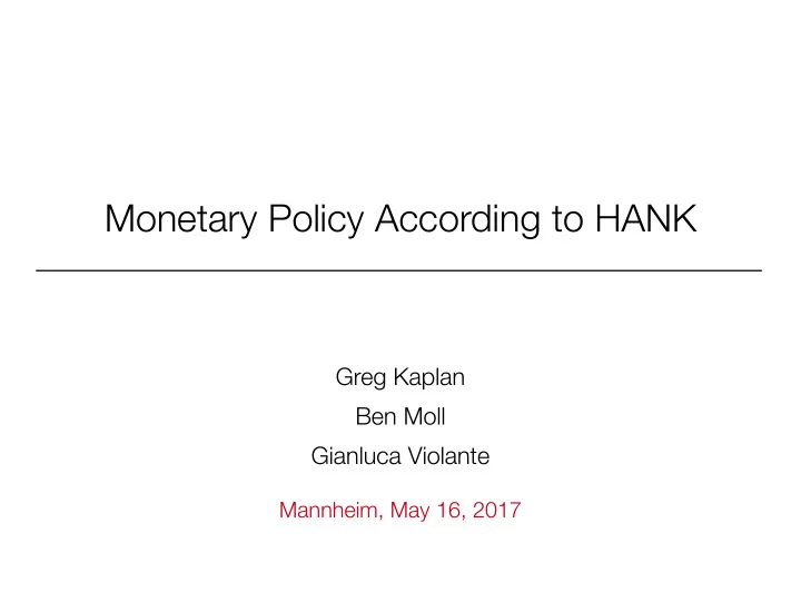
Monetary Policy According to HANK Greg Kaplan Ben Moll Gianluca - PowerPoint PPT Presentation

Monetary Policy According to HANK Greg Kaplan Ben Moll Gianluca Violante Mannheim, May 16, 2017

• Three building blocks 1. Uninsurable idiosyncratic income risk 2. Nominal price rigidities 3. Assets with different degrees of liquidity HANK: Heterogeneous Agent New Keynesian models • Framework for quantitative analysis of the transmission mechanism of monetary policy 1

HANK: Heterogeneous Agent New Keynesian models • Framework for quantitative analysis of the transmission mechanism of monetary policy • Three building blocks 1. Uninsurable idiosyncratic income risk 2. Nominal price rigidities 3. Assets with different degrees of liquidity 1

• However, data suggest: 1. Low sensitivity of to 2. Sizable sensitivity of to 3. Micro sensitivity vastly heterogeneous, depends crucially on household balance sheets How monetary policy works in RANK • Total consumption response to a drop in real rates C response = direct response to r + indirect effects due to Y � �� � � �� � <5% >95% • Direct response is everything, pure intertemporal substitution 2

How monetary policy works in RANK • Total consumption response to a drop in real rates C response = direct response to r + indirect effects due to Y � �� � � �� � <5% >95% • Direct response is everything, pure intertemporal substitution • However, data suggest: 1. Low sensitivity of C to r 2. Sizable sensitivity of C to Y 3. Micro sensitivity vastly heterogeneous, depends crucially on household balance sheets 2

response direct response to indirect effects due to RANK: >95% RANK: <5% HANK: <1/3 HANK: >2/3 • Overall effect depends crucially on fiscal response, unlike in RANK where Ricardian equivalence holds How monetary policy works in HANK • Once matched to micro data, HANK delivers realistic: • wealth distribution: small direct effect • MPC distribution: large indirect effect (depending on ∆ Y ) 3

• Overall effect depends crucially on fiscal response, unlike in RANK where Ricardian equivalence holds How monetary policy works in HANK • Once matched to micro data, HANK delivers realistic: • wealth distribution: small direct effect • MPC distribution: large indirect effect (depending on ∆ Y ) C response = direct response to r indirect effects due to Y � + � �� � � �� RANK: >95% RANK: <5% HANK: <1/3 HANK: >2/3 3

How monetary policy works in HANK • Once matched to micro data, HANK delivers realistic: • wealth distribution: small direct effect • MPC distribution: large indirect effect (depending on ∆ Y ) C response = direct response to r indirect effects due to Y � + � �� � � �� RANK: >95% RANK: <5% HANK: <1/3 HANK: >2/3 • Overall effect depends crucially on fiscal response, unlike in RANK where Ricardian equivalence holds 3

Closest existing work: 1. New Keynesian models with limited heterogeneity Campell-Mankiw, Gali-LopezSalido-Valles, Iacoviello, Bilbiie, Challe-Matheron-Ragot-Rubio-Ramirez • micro-foundation of spender-saver behavior 2. Bewley models with sticky prices Oh-Reis, Guerrieri-Lorenzoni, Ravn-Sterk, Gornemann-Kuester-Nakajima, DenHaan-Rendal-Riegler, Bayer-Luetticke-Pham-Tjaden, McKay-Reis, McKay-Nakamura-Steinsson, Huo-RiosRull, Werning, Luetticke • assets with different liquidity Kaplan-Violante • new view of individual earnings risk Guvenen-Karahan-Ozkan-Song • Continuous time approach Achdou-Han-Lasry-Lions-Moll Literature and contribution Combine two workhorses of modern macroeconomics: • New Keynesian models Gali, Gertler, Woodford • Bewley models Aiyagari, Bewley, Huggett 4

• Continuous time approach Achdou-Han-Lasry-Lions-Moll Literature and contribution Combine two workhorses of modern macroeconomics: • New Keynesian models Gali, Gertler, Woodford • Bewley models Aiyagari, Bewley, Huggett Closest existing work: 1. New Keynesian models with limited heterogeneity Campell-Mankiw, Gali-LopezSalido-Valles, Iacoviello, Bilbiie, Challe-Matheron-Ragot-Rubio-Ramirez • micro-foundation of spender-saver behavior 2. Bewley models with sticky prices Oh-Reis, Guerrieri-Lorenzoni, Ravn-Sterk, Gornemann-Kuester-Nakajima, DenHaan-Rendal-Riegler, Bayer-Luetticke-Pham-Tjaden, McKay-Reis, McKay-Nakamura-Steinsson, Huo-RiosRull, Werning, Luetticke • assets with different liquidity Kaplan-Violante • new view of individual earnings risk Guvenen-Karahan-Ozkan-Song 4

Literature and contribution Combine two workhorses of modern macroeconomics: • New Keynesian models Gali, Gertler, Woodford • Bewley models Aiyagari, Bewley, Huggett Closest existing work: 1. New Keynesian models with limited heterogeneity Campell-Mankiw, Gali-LopezSalido-Valles, Iacoviello, Bilbiie, Challe-Matheron-Ragot-Rubio-Ramirez • micro-foundation of spender-saver behavior 2. Bewley models with sticky prices Oh-Reis, Guerrieri-Lorenzoni, Ravn-Sterk, Gornemann-Kuester-Nakajima, DenHaan-Rendal-Riegler, Bayer-Luetticke-Pham-Tjaden, McKay-Reis, McKay-Nakamura-Steinsson, Huo-RiosRull, Werning, Luetticke • assets with different liquidity Kaplan-Violante • new view of individual earnings risk Guvenen-Karahan-Ozkan-Song • Continuous time approach Achdou-Han-Lasry-Lions-Moll 4

• Budget constraints (simplified version) : liquid assets : illiquid assets : illiquid deposits ( ) : transaction cost function • In equilibrium: • Full model: borrowing/saving rate wedge, taxes/transfers HANK: a framework for monetary policy analysis Households • Face uninsured idiosyncratic labor income risk • Consume and supply labor • Hold two assets: liquid and illiquid 5

• Full model: borrowing/saving rate wedge, taxes/transfers HANK: a framework for monetary policy analysis Households • Face uninsured idiosyncratic labor income risk • Consume and supply labor • Hold two assets: liquid and illiquid • Budget constraints (simplified version) ˙ b t = r b b t + wz t ℓ t − c t − d t − χ ( d t , a t ) a t = r a a t + d t ˙ • b t : liquid assets • a t : illiquid assets • d t : illiquid deposits ( ≷ 0 ) • χ : transaction cost function • In equilibrium: r a > r b 5

HANK: a framework for monetary policy analysis Households • Face uninsured idiosyncratic labor income risk • Consume and supply labor • Hold two assets: liquid and illiquid • Budget constraints (simplified version) ˙ b t = r b b t + wz t ℓ t − c t − d t − χ ( d t , a t ) a t = r a a t + d t ˙ • b t : liquid assets • a t : illiquid assets • d t : illiquid deposits ( ≷ 0 ) • χ : transaction cost function • In equilibrium: r a > r b • Full model: borrowing/saving rate wedge, taxes/transfers 5

Kinked adjustment cost function χ ( d, a ) 6

Remaining model ingredients Illiquid assets: a = k + qs • No arbitrage: r k − δ = Π+ ˙ q := r a q Firms • Monopolistic intermediate-good producers → final good • Rent illiquid capital and labor services from hh • Quadratic price adjustment costs à la Rotemberg (1982) Government • Issues liquid debt ( B g ) , spends ( G ) , taxes and transfers ( T ) Monetary Authority • Sets nominal rate on liquid assets based on a Taylor rule 7

Summary of market clearing conditions • Liquid asset market B h + B g = 0 • Illiquid asset market A = K + q • Labor market ∫ N = zℓ ( a, b, z ) dµ • Goods market: Y = C + I + G + χ + Θ + borrowing costs 8

Solution Method 9

Solution Method (from Achdou-Han-Lasry-Lions-Moll) • Solving het. agent model = solving PDEs 1. Hamilton-Jacobi-Bellman equation for individual choices 2. Kolmogorov Forward equation for evolution of distribution • Many well-developed methods for analyzing and solving these • simple but powerful: finite difference method • codes: http://www.princeton.edu/~moll/HACTproject.htm • Apparatus is very general: applies to any heterogeneous agent model with continuum of atomistic agents 1. heterogeneous households (Aiyagari, Bewley, Huggett,...) 2. heterogeneous producers (Hopenhayn,...) • can be extended to handle aggregate shocks (Krusell-Smith,...) 10

Computational Advantages relative to Discrete Time 1. Borrowing constraints only show up in boundary conditions • FOCs always hold with “ = ” 2. “Tomorrow is today” • FOCs are “static”, compute by hand: c − γ = V b ( a, b, y ) 3. Sparsity • solving Bellman, distribution = inverting matrix • but matrices very sparse (“tridiagonal”) • reason: continuous time ⇒ one step left or one step right 4. Two birds with one stone • tight link between solving (HJB) and (KF) for distribution • matrix in discrete (KF) is transpose of matrix in discrete (HJB) • reason: diff. operator in (KF) is adjoint of operator in (HJB) 11

HA Models with Aggregate Shocks: A Matlab Toolbox • Achdou et al & HANK: HA models with idiosyncratic shocks only • Aggregate shocks ⇒ computational challenge much larger • Companion project: efficient, easy-to-use computational method • see “When Inequality Matters for Macro and Macro Matters for Inequality” (with Ahn, Kaplan, Winberry and Wolf) • open source Matlab toolbox online now – see my website and https://github.com/gregkaplan/phact • extension of linearization (Campbell 1998, Reiter 2009) • different slopes at each point in state space 12

Parameterization 13