Modelling Dependent Credit Risks Advanced Mathematical Methods for - PowerPoint PPT Presentation
Workshop and Mid-Term Conference on Modelling Dependent Credit Risks Advanced Mathematical Methods for Finance with Extensions of CreditRisk + (Mid-Term AMaMeF Meeting 2007) and Application to Operational Risk September 1823, 2007, Vienna,
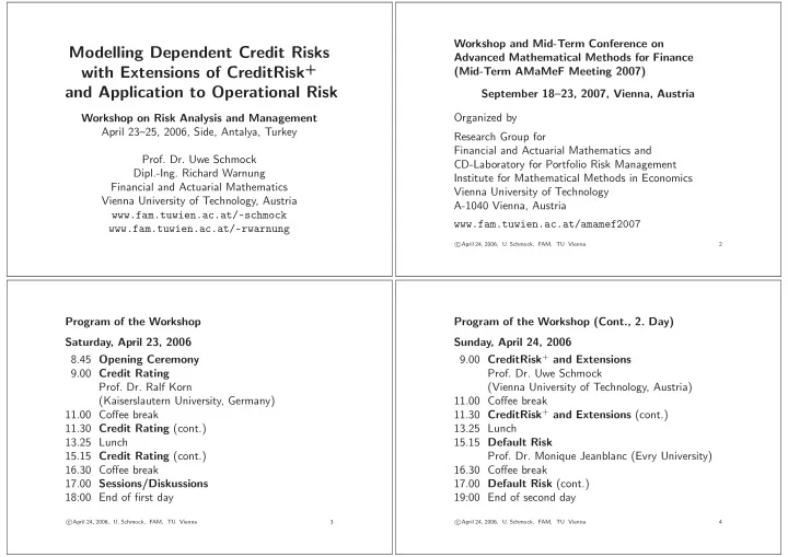
Workshop and Mid-Term Conference on Modelling Dependent Credit Risks Advanced Mathematical Methods for Finance with Extensions of CreditRisk + (Mid-Term AMaMeF Meeting 2007) and Application to Operational Risk September 18–23, 2007, Vienna, Austria Workshop on Risk Analysis and Management Organized by April 23–25, 2006, Side, Antalya, Turkey Research Group for Financial and Actuarial Mathematics and Prof. Dr. Uwe Schmock CD-Laboratory for Portfolio Risk Management Dipl.-Ing. Richard Warnung Institute for Mathematical Methods in Economics Financial and Actuarial Mathematics Vienna University of Technology Vienna University of Technology, Austria A-1040 Vienna, Austria www.fam.tuwien.ac.at/~schmock www.fam.tuwien.ac.at/amamef2007 www.fam.tuwien.ac.at/~rwarnung c � April 24, 2006, U. Schmock, FAM, TU Vienna 2 Program of the Workshop Program of the Workshop (Cont., 2. Day) Saturday, April 23, 2006 Sunday, April 24, 2006 9.00 CreditRisk + and Extensions 8.45 Opening Ceremony 9.00 Credit Rating Prof. Dr. Uwe Schmock Prof. Dr. Ralf Korn (Vienna University of Technology, Austria) (Kaiserslautern University, Germany) 11.00 Coffee break 11.30 CreditRisk + and Extensions (cont.) 11.00 Coffee break 11.30 Credit Rating (cont.) 13.25 Lunch 13.25 Lunch 15.15 Default Risk 15.15 Credit Rating (cont.) Prof. Dr. Monique Jeanblanc (Evry University) 16.30 Coffee break 16.30 Coffee break 17.00 Sessions/Diskussions 17.00 Default Risk (cont.) 18:00 End of first day 19:00 End of second day c c � April 24, 2006, U. Schmock, FAM, TU Vienna 3 � April 24, 2006, U. Schmock, FAM, TU Vienna 4
Program of the Workshop (Cont., 3. Day) Monday, April 25, 2006 Introduction to 9.00 CreditRisk + and Extensions Credit Risk Modelling Prof. Dr. Uwe Schmock (TU Vienna) 11.00 Coffee break 11.30 Sessions/Diskussions 13.25 Lunch 15.15 Default Risk Prof. Dr. Uwe Schmock Prof. Dr. Monique Jeanblanc (Evry University) Director of PRisMa Lab 16.30 Coffee break Financial and Actuarial Mathematics 17.00 Sessions/Diskussions Vienna University of Technology, Austria 19:00 Closing Ceremony www.fam.tuwien.ac.at/ ∼ schmock www.prismalab.at c c � April 24, 2006, U. Schmock, FAM, TU Vienna 5 � April 24, 2006, U. Schmock, FAM, TU Vienna 6 Components of Credit Risk Components of Credit Risk (Cont.) • Arrival risk: Uncertainty whether a default will • Rating transition risk: Risk of changing market price occur or not. Measured by the probability of default, of a defaultable security due to a changed perception within a given time horizon, usually one year. of the market towards the timing or recovery risk • Timing risk: Uncertainty about the time of default. (without an actual default already happening). • Exposure risk: Relatively clear for loans or bonds It often happens together with an up- or down-rating (face value, market value), greater uncertainty in the of the creditworthiness by a rating agency. credit reinsurance business as primary insurers might • Default correlation risk: Risk of several obligors have successfully decreased credit lines in advance. defaulting together; leads to substantial losses even • Recovery risk: Uncertainty about the size of the loss in well diversified portfolios. Defaults in investment- w.r.t. the exposure. Historical data show a large grade rating classes are rare, hence it is hard to variability of recovery rate, depending on collateral, collect data to estimate the dependence of defaults. seniority of the bond, etc. Specified by conditional distribution of recovery rate given default occurred. c c � April 24, 2006, U. Schmock, FAM, TU Vienna 7 � April 24, 2006, U. Schmock, FAM, TU Vienna 8
Time Series versus Default Modelling Credit Ratings for Bonds Time series modelling (e.g. exchange rates) A credit rating is a current opinion of an obligor’s overall financial capacity (its creditworthiness) to pay • Collect data for a long time (e.g. CHF/US-$). its financial obligations. • Assume stationarity of stochastic behaviour, fit a suitable model (random walk, GARCH, etc.) Standard & Poor’s Investor Services and make predictions about the future. Investment grade: AAA, AA, A, BBB Default modelling Speculative: BB, B, CCC, CC, C (D = Default) • Observing a firm until today doesn’t give a default AA–B: + = above, − = below average in rating class observation ( → observation bias). Moody’s Investor Services • Solution: Observe a group of firms, draw conclusions for a specific firm. Investment grade: Aaa, Aa, A • Problems: Relevance of data for the specific firm? Speculative: Baa, Ba, B, Caa, Ca, C When are firms similar w.r.t. creditworthiness? Aa–B: 1 = above, 2 = at, 3 = below average in rating class c c � April 24, 2006, U. Schmock, FAM, TU Vienna 9 � April 24, 2006, U. Schmock, FAM, TU Vienna 10 Some Offered Bonds July 2004 (in CHF) Some Current Bonds (in USD) Matur- Rating Matur- Rating Company Coupon ity Price S & P Moody’s Date Company Coupon ity Price S & P Moody’s YTM WestLB ∗ float 28.7.06 100.060 AA Aa2 22.7. Daimler Chr. NA 6.400 15.5.06 100.194 BBB A3 6.292 GECC † float 23.7.07 100.070 AAA Aaa 20.7. AT & T 7.500 1.6.06 100.193 A Baa2 5.398 Commonwealth Wal Mart Stores 5.450 1.8.06 100.231 AA Aa2 4.506 Bank of Australia 1.750 4.9.07 100.085 AA– Aa3 30.7. Time Warner 8.110 15.8.06 100.794 BBB+ Baa2 5.384 Principal Financial Global Funding 2.750 12.7.10 100.190 AA Aa3 8.7. Citigroup Inc. 5.500 8.9.06 100.271 AA − Aa1 4.486 Sigma Finance 2.375 29.7.11 100.225 AAA Aaa 21.7. HP Co. 5.750 15.12.06 100.334 A − A3 5.2 Hypo Tirol Bank 3.000 20.11.12 101.600 AAA 5.8. Source: www.bonddesk.com April 21, 2006 ∗ 3-month Libor flat † 3-month Libor + 2 bp Neue Z¨ urcher Zeitung (NZZ, Vol. 225), July 7, 2004 c c � April 24, 2006, U. Schmock, FAM, TU Vienna 11 � April 24, 2006, U. Schmock, FAM, TU Vienna 12
Merton Model Classification of Credit Risk Models • Firm-value (or structural) models 200 Assets of the firm Pioneered by Black & Scholes (1973), Merton (1974) Industry models: Portfolio Manager (by KMV), 150 CreditMetrics (RiskMetrics Group) A t • Intensity-based (or reduced-form) models 100 Jarrow & Turnbull (1995), Liabilities of L = 100 Jarrow, Lando & Turnbull (1997), Lando (1996, 1998), Duffie & Singleton (1999) 50 • Actuarial models Mixture models, CreditRisk + (CS Financial Products) Years 0 0 1 2 3 4 • Macroeconomic models Exponential Brownian motion A t = 200 exp(0 . 3 W t ). Industry: CreditPortfolioView (McKinsey & Company) Default occures when A t < L . c c � April 24, 2006, U. Schmock, FAM, TU Vienna 13 � April 24, 2006, U. Schmock, FAM, TU Vienna 14 Classification of Credit Risk Models Discrete-Time Motivation for Intensity Models • Firm-value (or structural) models Time Pioneered by Black & Scholes (1973), Merton (1974) 0 1 . . . t t + 1 t + 2 . . . T Industry models: Portfolio Manager (by KMV), Notation CreditMetrics (RiskMetrics Group) X promised (but defaultable) payout at time T • Intensity-based (or reduced-form) models h t conditional probability at time t Jarrow & Turnbull (1995), for default during the period [ t, t + 1] Jarrow, Lando & Turnbull (1997), r t continuously compounded, default-free Lando (1996, 1998), Duffie & Singleton (1999) interest rate for the period [ t, t + 1] • Actuarial models ϕ t +1 random recovery at t + 1 in case Mixture models, CreditRisk + (CS Financial Products) of default during [ t, t + 1] • Macroeconomic models E Q [ ·|F t ] conditional expectation under Q Industry: CreditPortfolioView (McKinsey & Company) given all the information F t up to time t c c � April 24, 2006, U. Schmock, FAM, TU Vienna 15 � April 24, 2006, U. Schmock, FAM, TU Vienna 16
Evolution of Market Value V t Different Assumptions for the Recovery ϕ t +1 (recovery) Recovery of face value: ϕ t = 1 − L t h t The creditor receives a (possible random) fraction of Time t V t Time t + 1 the face value 1 immediately upon default. 1 − h t Recovery of treasury: ϕ t = (1 − L t ) P ( t, T ) V t +1 The creditor receives a (possible random) fraction of Recursion formula a corresponding default-free government bond. V t = h t e − r t E Q [ ϕ t +1 |F t ] + (1 − h t ) e − r t E Q [ V t +1 |F t ] Recovery of market value (RMV): E Q [ ϕ t +1 |F t ] = (1 − L t ) E Q [ V t +1 |F t ] with terminal value V T = X . The expected recovery is a (random) fraction of the An explicit formula for V 0 by backward induction is expected market value in case of no default. available but complicated to evaluate. c c � April 24, 2006, U. Schmock, FAM, TU Vienna 17 � April 24, 2006, U. Schmock, FAM, TU Vienna 18 Distribution of Recovery by Seniority Transition to Hazard and Loss Rates Percentage of face value in secondary market after default 100 With recovery of market value 90 80 90% quantile V t = { (1 − h t ) e − r t + h t e − r t (1 − L t ) } E Q [ V t +1 |F t ] median 70 � �� � central 50% =: e − Rt 60 10% quantile 50 with e − R t = (1 − h t L t ) e − r t ≈ e − ( r t + h t L t ) , because 40 � 1 − h t � n 30 → e − h t L t n L t n → ∞ . 20 10 n is the number of subdivisions per period. Hence Bank Senior Secured Senior Subordinated Junior � � e − ( R 0 + ··· + R T − 1 ) X V 0 = E Q . Loans Unsecured Bonds Subordinated Bonds Bonds Bonds Based on Moody’s data 1974–1997 c c � April 24, 2006, U. Schmock, FAM, TU Vienna 19 � April 24, 2006, U. Schmock, FAM, TU Vienna 20
Recommend
More recommend
Explore More Topics
Stay informed with curated content and fresh updates.

