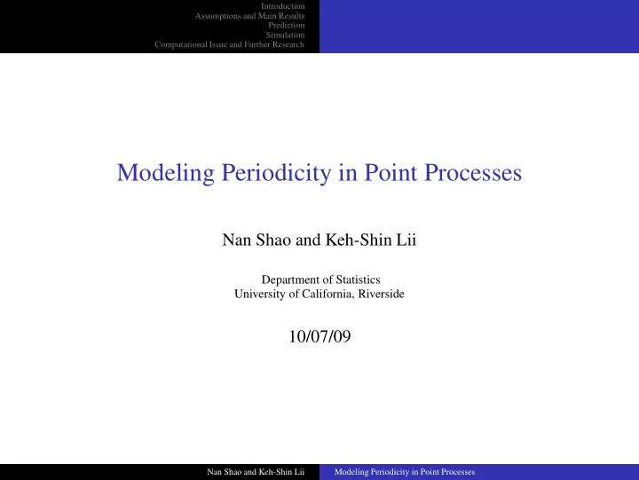
Modeling Periodicity in Point Processes Nan Shao and Keh-Shin Lii - PowerPoint PPT Presentation
Introduction Assumptions and Main Results Prediction Simulation Computational Issue and Further Research Modeling Periodicity in Point Processes Nan Shao and Keh-Shin Lii Department of Statistics University of California, Riverside 10/07/09
Introduction Assumptions and Main Results Prediction Simulation Computational Issue and Further Research Modeling Periodicity in Point Processes Nan Shao and Keh-Shin Lii Department of Statistics University of California, Riverside 10/07/09 Nan Shao and Keh-Shin Lii Modeling Periodicity in Point Processes
Introduction Assumptions and Main Results Prediction Simulation Computational Issue and Further Research Outline Introduction Motivation and Basic Concept of Point Process A Brief Review and Our Model Assumptions and Main Results Assumptions Estimation of the Parameters Prediction Simulation Computational Issue and Further Research 2 / 49
Introduction Assumptions and Main Results Motivation and Basic Concept of Point Process Prediction A Brief Review and Our Model Simulation Computational Issue and Further Research Point Process Point processes arise when events occur at random times. ◮ Initiation of phone calls at a service center. ◮ Earthquake in certain area. ◮ The arrival of ambulance at ER. ◮ Stock transactions. 3 / 49
Introduction Assumptions and Main Results Motivation and Basic Concept of Point Process Prediction A Brief Review and Our Model Simulation Computational Issue and Further Research Periodic Point Processes ◮ Stock transaction with daily cycle. ◮ Weekly effect in phone calls at customer center. ◮ Imoto et al. (1999) discussed the periodic pattern of seismicity observed in central Japan. 4 / 49
Introduction Assumptions and Main Results Motivation and Basic Concept of Point Process Prediction A Brief Review and Our Model Simulation Computational Issue and Further Research Definition of Point Process ◮ Let { t i , i = 1 , 2 , . . . } be a sequence of nonnegative random variables on a probability space (Ω , F , P ) with 0 ≤ t i ≤ t i + 1 , then the sequence { t i } is called a point process on [ 0 , ∞ ] . ◮ If there is no multiple occurrence, namely, t i < t i + 1 for any i , the process is called a simple point process . We will restrict out attention to simple point process. ◮ Let the sequence { t 1 , t 2 , . . . } be a point process. Let N ( s , t ) be the number of points in time interval ( s , t ] , and denote N ( t ) = N ( 0 , t ) . Then N ( t ) is called a counting process . 5 / 49
Introduction Assumptions and Main Results Motivation and Basic Concept of Point Process Prediction A Brief Review and Our Model Simulation Computational Issue and Further Research Intensity Function The intensity function λ ( t ) of a point process, also called the mean rate of occurrence in Cox and Isham (1980), is defined as P { N ( t , t + δ ) > 0 } λ ( t ) = lim δ δ → 0 + E { N ( t , t + δ ) } = lim . δ δ → 0 + So E { dN ( t ) } = λ ( t ) dt . It describes the first-order moment property of the unconditional counting measure. 6 / 49
Introduction Assumptions and Main Results Motivation and Basic Concept of Point Process Prediction A Brief Review and Our Model Simulation Computational Issue and Further Research 3 2 intensity 1 0 0 10 20 30 40 50 60 time Figure: Solid line: the intensity function of a non-homogeneous Poisson process λ ( t ) = cos ( 3 t ) + 0 . 5 cos ( 2 t + π π π 4 ) + 1 . 6. Triangle points: the occurrence time √ √ 4 3 of events. 7 / 49
Introduction Assumptions and Main Results Motivation and Basic Concept of Point Process Prediction A Brief Review and Our Model Simulation Computational Issue and Further Research A Brief Review ◮ Lewis (1970, 1972) established the estimation and detection of a cyclic varying rate of a non-homogeneous Poisson process when the frequency is known a priori . The rate function took the following form λ ( t ) = A exp { ρ cos ( ω t + φ ) } . Vere-Jones (1982) proposed a method to estimate the frequency ω in above model and established its asymptotic property. ◮ Helmers et al. (2003) constructed a consistent kernel-type nonparametric estimate of the intensity function of a cyclic Poisson process where the intensity function is cyclic with only one period and the period is unknown. 8 / 49
Introduction Assumptions and Main Results Motivation and Basic Concept of Point Process Prediction A Brief Review and Our Model Simulation Computational Issue and Further Research Almost Periodic Point Processes ◮ General idea on ‘almost periodic’: any particular configuration that occurs once may recur not exactly, but within some accuracy. ◮ A sequence which appears to be ‘chaotic’ and ‘uninformative’ is a superstition of several periodic components and it is almost periodic. ◮ Almost periodic point process is much more general than the periodic one. 3.0 2.5 2.0 intensity 1.5 1.0 0.5 0.0 0 20 40 60 80 100 t Figure: Almost periodic function λ ( t ) = cos ( 3 t ) + 0 . 5 cos ( 2 t + π π π 4 ) + 1 . 6. √ √ 4 3 9 / 49
Introduction Assumptions and Main Results Motivation and Basic Concept of Point Process Prediction A Brief Review and Our Model Simulation Computational Issue and Further Research Our Model The intensity function we consider is of the form K � λ ( t ) = A k cos ( ω k t + φ k ) + B , (1) i = 1 where A k , B , ω k , φ k are unknown parameters with A 1 > A 2 > · · · > A K > 0, � K k = 1 A k < B , 0 ≤ φ k < 2 π and ω k > 0, k = 1 , . . . , K . 10 / 49
Introduction Assumptions and Main Results Motivation and Basic Concept of Point Process Prediction A Brief Review and Our Model Simulation Computational Issue and Further Research Periodogram Periodogram in point processes is defined by Bartlett (1963) as follows I T ( ω ) = d T ( ω ) d T ( ω ) , where ( 0 , T ) is the observation interval, and d T ( ω ) is the finite Fourier transform , defined as � T 1 e − i ω t dN ( t ) d T ( ω ) = √ 2 π T 0 N ( t ) 1 e − i ω t j . � √ = 2 π T j = 1 11 / 49
Introduction Assumptions and Main Results Motivation and Basic Concept of Point Process Prediction A Brief Review and Our Model Simulation Computational Issue and Further Research 15 10 periodogram 5 0 0 1 2 3 4 5 ω Figure: The periodogram of a non-homogeneous Poisson process with intensity function λ ( t ) = cos ( 3 t ) + 0 . 5 cos ( 2 t + π π π 4 ) + 1 . 6. The process consists 778 √ √ 4 3 observations with observation length T = 500. 12 / 49
Introduction Assumptions and Main Results Assumptions Prediction Estimation of the Parameters Simulation Computational Issue and Further Research Assumptions ◮ Assumption 1 N ( t ) , t ≥ 0, is a non-homogeneous Poisson process with a periodic or almost periodic intensity function (1), observed over the time interval [ 0 , T ] , and the number of periodic components K is given. ◮ Minimum separation: Assumption 2 T min k � = k ′ ( | ω k − ω k ′ | ) → ∞ , as T → ∞ . ◮ Searching range: Assumption 3 O ( T δ ′ − 1 ) ≤ ω k ≤ Ω T , k = 1 , . . . , K , where 0 < δ ′ < 1 and Ω T is the upper bound, possibly determined by observations on the process in the interval ( 0 , T ) with E (Ω T ) = O ( T 1 − δ ) , δ > 0. 13 / 49
Introduction Assumptions and Main Results Assumptions Prediction Estimation of the Parameters Simulation Computational Issue and Further Research Estimation of the Frequencies Let ω = ( ω 1 , . . . , ω K ) ′ , we determine ˆ ω T as frequencies corresponding to the K largest local maxima of the periodogram in the range defined in Assumption 3 and the corresponding frequencies are well separated where their shortest distance cannot decrease sufficiently faster than O ( T − 1 ) as T → ∞ . 15 periodogram 10 5 0 0 1 2 3 4 5 ω Figure: The periodogram of a non-homogeneous Poisson process with intensity function λ ( t ) = cos ( 3 t ) + 0 . 5 cos ( 2 t + π π π 4 ) + 1 . 6. The process consists 778 √ √ 4 3 observations with observation length T = 500. 14 / 49
Introduction Assumptions and Main Results Assumptions Prediction Estimation of the Parameters Simulation Computational Issue and Further Research 15 10 periodogram 5 [ ] 0 0 1 2 3 4 5 ω 15 / 49
Introduction Assumptions and Main Results Assumptions Prediction Estimation of the Parameters Simulation Computational Issue and Further Research 15 10 periodogram 5 [ ] 0 0 1 2 3 4 5 ω 16 / 49
Introduction Assumptions and Main Results Assumptions Prediction Estimation of the Parameters Simulation Computational Issue and Further Research Super Efficiency of ˆ ω T Proposition 1 Under Assumptions 1, 2 and 3, ˆ ω T is a consistent estimate of ω , and ω k , T − ω k ) = o ( T − 1 ) , ( a . s . ) , k = 1 , . . . , K . (ˆ 17 / 49
Recommend
More recommend
Explore More Topics
Stay informed with curated content and fresh updates.
