Mining Data Graphs Semi-supervised learning, label propagation, Web - PowerPoint PPT Presentation
Mining Data Graphs Semi-supervised learning, label propagation, Web Search Data graphs Data graphs are common in Web data Web link graph Chains of discussions It is also possible to create data graphs from Web data Using
Mining Data Graphs Semi-supervised learning, label propagation, Web Search
Data graphs • Data graphs are common in Web data • Web link graph • Chains of discussions • It is also possible to create data graphs from Web data • Using similarity methods between data elements • Graphs from Web data • The graph vertices are the elements we whish to analyse • The graph edges capture the level of affinity between two of such elements 2
However, in Web domain… • I have a good idea, but I can’t afford to label lots of data! • I have lots of labeled data, but I have even more unlabeled data • It’s not just for small amounts of labeled data anymore! 3
What is semi-supervised learning (SSL)? • Labeled data (entity classification) Labels person • …, says Mr. Cooper , vice location president of … organization • … Firing Line Inc., a Philadelphia gun shop. • Lots more unlabeled data • …, Yahoo’s own Jerry Yang is right … • … The details of Obama’s San Francisco mis- adventure … 4
Graph-based semi-supervised Learning • From items to graphs • Basic graph-based algorithms • Mincut • Label propagation • Graph consistency 5
Text classification: easy example • Two classes: astronomy vs. travel • Document = 0-1 bag-of-word vector • Cosine similarity x1=“bright asteroid”, y1=astronomy Easy, by x2=“yellowstone denali”, y2=travel x3=“asteroid comet”? word x4=“camp yellowstone”? overlap 6
Hard example x1=“bright asteroid”, y1=astronomy x2=“yellowstone denali”, y2=travel x3=“zodiac”? x4=“airport bike”? • No word overlap • Zero cosine similarity • Pretend you don’t know English 7
Hard example x1 x3 x4 x2 asteroid 1 bright 1 comet zodiac 1 airport 1 bike 1 yellowstone 1 denali 1 8
Unlabeled data comes to the rescue x1 x5 x6 x7 x3 x4 x8 x9 x2 asteroid 1 bright 1 1 1 comet 1 1 1 zodiac 1 1 airport 1 bike 1 1 1 yellowstone 1 1 1 denali 1 1 9
Intuition 1. Some unlabeled documents are similar to the labeled documents same label 2. Some other unlabeled documents are similar to the above unlabeled documents same label 3. ad infinitum We will formalize this with graphs . 10
The graph • Nodes 𝑦 1 , … , 𝑦 𝑚 ∪ 𝑦 𝑚+1 , … , 𝑦 𝑛+𝑚 • Weighted, undirected edges 𝑥 𝑗𝑘 • Large weight similar 𝑦 𝑗 , 𝑦 𝑘 d1 • Known labels 𝑧 1 , … , 𝑧 𝑚 d3 d2 • Want to know • transduction: 𝑧 𝑚+1 , … , 𝑧 𝑛+𝑚 • induction: y ∗ for new test item x ∗ d4 11
How to create a graph 1. Compute distance between i, j 2 𝑥 𝑗𝑘 = exp − 𝑦 𝑗 − 𝑦 𝑘 2𝜏 2 2. For each i, connect to its kNN. k very small but still connects the graph 3. Optionally put weights on (only) those edges 4. Tune 12
Mincut (s-t cut) • Binary labels 𝑧 𝑗 ∈ 0,1 . • Fix 𝑍 𝑚 = 𝑧 1 , … , 𝑧 𝑚 • Solve for 𝑍 𝑣 = 𝑧 𝑚+1 , … , 𝑧 𝑚+𝑛 𝑜 2 min 𝑥 𝑗,𝑘 𝑧 𝑗 − 𝑧 𝑘 𝑍 𝑣 𝑗,𝑘=1 • Combinatorial problem (integer program) but efficient polynomial time solver (Boykov, Veksler, Sabih PAMI 2001). 13
Mincut example: Opinion detection • Task: classify each sentence in a document into objective / subjective . (Pang,Lee. ACL 2004) • NB/SVM for isolated classification • Subjective data (y=1): Movie review snippets “bold, imaginative, and impossible to resist” • Objective data (y=0): IMDB 14
Mincut example: Opinion detection • Key observation: sentences next to each other tend to have the same label • Two special labeled nodes (source, sink) • Every sentence connects to both with different weight 15
Opinion detection • Min cut classifies sentences as subjective vs objective. • Impact on the detection of opinion positive/negative: 16
Mincut example (s-t cut) 17
Some issues with mincut • Multiple equally min cuts, but different in practice: • Lacks classification confidence • These are addressed by harmonic functions and label propagation 18
Relaxing mincut • Labels are now real values in the interval [0,1] 𝑔 𝑦 𝑚 = 𝑧 𝑚 𝑜 2 min 𝑥 𝑗,𝑘 𝑔 𝑗 − 𝑔 𝑘 𝑔 𝑣 𝑗,𝑘=1 • Same as mincut except that 𝑔 𝑣 ∈ 𝑆 • 𝑔 𝑣 ∈ 0,1 and is less confident near 0.5 19
An electric network interpretation 1 R = ij w 1 ij +1 volt 0 20
Label propagation • Algorithm: Set 𝑔 𝑣 = 0 1. Set 𝑔 𝑚 = 𝑧 𝑚 . 2. 𝑜 σ 𝑙=1 𝑥 𝑙𝑣 ⋅𝑔 𝑙 3. Propagate: 𝑔 𝑣 = 𝑥 𝑙𝑣 . 𝑜 σ 𝑙=1 4. Row normalize f 5. Repeat from step 2 21
Label propagation example: WSD • Word sense disambiguation from context, e.g., “interest”, “line” ( Niu,Ji,Tan ACL 2005) • x i : context of the ambiguous word, features: POS, words, collocations • d ij : cosine similarity or JS-divergence • w ij : kNN graph • Labeled data: a few x i ’s are tagged with their word sense. 24
Label propagation example: WSD • SENSEVAL-3, as percent labeled: (Niu,Ji,Tan ACL 2005) 25
Graph consistency • The key to semi-supervised learning problems is the prior assumption of consistency: • Local Consistency : nearby points are likely to have the same label; • Global Consistency : Points on the same structure (cluster or manifold) are likely to have the same label; 26
Local and Global Consistency • The key to the consistency algorithm is to let every point iteratively spread its label information to its neighbors until a global stable state is achieved. 27
Definitions • Data points: 𝑦 1 , … , 𝑦 𝑚 ∪ 𝑦 𝑚+1 , … , 𝑦 n • Label set: 𝑀 = 1, … , 𝑑 • Y is the initial classification on 𝑦 1 , … , 𝑦 𝑚 with: 𝑗𝑘 = ቊ 1, 𝑗𝑔 𝑦 𝑗 𝑗𝑡 𝑚𝑏𝑐𝑓𝑚𝑓𝑒 𝑏𝑡 𝑧 𝑗 = 𝑘 𝑍 0, 𝑝𝑢ℎ𝑓𝑠𝑥𝑗𝑡𝑓 • F, a classification on x: 𝐺 … 𝐺 11 1𝑑 … … … 𝐺 𝑜×𝑑 = 𝐺 … 𝐺 𝑜1 𝑜𝑑 ∗ Labeling 𝑦 𝑚+1 , … , 𝑦 n as y i = argmax 𝑘≤𝑑 𝐺 𝑗𝑘 28
Consistency algorithm: the graph 1. Construct the affinity matrix W defined by a Gaussian kernel: 2 𝑥 𝑗𝑘 = ൞exp − 𝑦 𝑗 − 𝑦 𝑘 , 𝑗𝑔 𝑗 ≠ 𝑘 2𝜏 2 0 𝑗𝑔 𝑗 = 𝑘 2. Normalize W symmetrically by 𝑇 = 𝐸 −1/2 𝑋𝐸 −1/2 where D is a diagonal matrix with 𝐸 𝑗𝑗 = σ 𝑙 𝑥 𝑗𝑙 29
Consistency algorithm: the propagation 3. Iterate until convergence: 𝐺 𝑢 + 1 = 𝛽 ⋅ 𝑇 ⋅ 𝐺 𝑢 + 1 − 𝛽 ⋅ 𝑍 • First term : each point receive information from its neighbors. • Second term : retains the initial information. • Normalize F on each iteration. 4. Let 𝐺 ∗ denote the limit of the sequence {F(t)}. The classification results are: ∗ Labeling x i as y i = argmax 𝑘≤𝑑 𝐺 𝑗𝑘 30
Closed-form solution • From the iteration equation, we can show that: 𝐺 ∗ = lim 𝑢→∞ 𝐺 𝑢 = 𝐽 − 𝛽𝑇 −1 ⋅ Y • So we could compute F* directly without iterations. • The closed-form may be too complex to calculate for very large graphs (the matrix inversion step) 31
The convergence process • The initial label information are diffused along the two moons. 32
Experimental Results Text classification : topics including Digit recognition : digit 1-4 from the autos, motorcycles, baseball and USPS data set hockey from the 20-newsgroups 33
Caution • Advantages of graph-based methods: • Clear intuition, elegant math • Performs well if the graph fits the task • Disadvantages: • Performs poorly if the graph is bad: sensitive to graph structure and edge weights • Usually we do not know which will happen! 34
Conclusions • The key to semi-supervised learning problem is the consistency assumption. • The consistency algorithm proposed was demonstrated effective on the data set considered. 35
Recommend
More recommend
Explore More Topics
Stay informed with curated content and fresh updates.
