Minimum Power Dominating Sets of Random Cubic Graphs - PowerPoint PPT Presentation
Minimum Power Dominating Sets of Random Cubic Graphs Liying Kang Dept. of
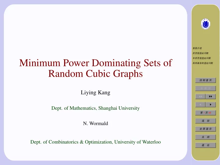
✒ ➭✵ ☛ � ✝ ✳➚ ➀ ➥ ❑ ➀ � ✝ ✳➚ ➀ ➥ ❑ Minimum Power Dominating Sets of ä ❦ ✗ ➦ ✛ ➚ ➀ ➥ ❑ Random Cubic Graphs ↔ ✔ ➘ ➄ ■ ❑ ➄ Liying Kang ◭◭ ◮◮ ◭ ◮ Dept. of Mathematics, Shanghai University ✶ 1 ➄ 55 ❼ ↔ N. Wormald ✜ ➯ ✇ ➠ ✬ ✹ Dept. of Combinatorics & Optimization, University of Waterloo ò Ñ
Outline ✒ ➭✵ ☛ � ✝ ✳➚ ➀ ➥ ❑ � 1 Introduction ➀ � ✝ ✳➚ ➀ ➥ ❑ ä ❦ ✗ ➦ ✛ ➚ ➀ ➥ ❑ � 2 Lower Bound for all Cubic Graphs via Bisection Width ↔ ✔ ➘ ➄ � ■ ❑ ➄ 3 Random Graphs and Differential Equations ◭◭ ◮◮ � ◭ ◮ 4 Algorithm PD1 and an Upper Bound ✶ 2 ➄ 55 � ❼ ↔ 58 Algorithm PD2 and an Upper Bound ✜ ➯ ✇ ➠ ✬ ✹ ò Ñ
1 Introduction ✒ ➭✵ ☛ � ✝ ✳➚ ➀ ➥ ❑ ➀ � ✝ ✳➚ ➀ ➥ ❑ Power Domination Problem ä ❦ ✗ ➦ ✛ ➚ ➀ ➥ ❑ Let G be a connected graph and S a subset of its vertices. Denote by M ( S ) the set monitored by S , defined algorithmically as follows: ↔ ✔ ➘ ➄ 1. ( domination) ■ ❑ ➄ M ( S ) ← S ∪ N ( S ) ◭◭ ◮◮ 2. ( propagation) ◭ ◮ If there exist any v ∈ M ( S ) and w / ∈ M ( S ) such that ✶ 3 ➄ 55 N ( v ) \ M ( S ) = { w } choose any such w and set M ( S ) ← M ( S ) ∪ { w } . ❼ ↔ ✜ ➯ ✇ ➠ ✬ ✹ ò Ñ
✒ ➭✵ ☛ � ✝ ✳➚ ➀ ➥ ❑ In other words, the set M ( G ) is obtained from S as follows. First put into M ( S ) ➀ � ✝ ✳➚ ➀ ➥ ❑ the vertices from the closed neighbourhood of S . Then repeatedly add to M ( S ) ä ❦ ✗ ➦ ✛ ➚ ➀ ➥ ❑ any vertex w that has a neighbour v in M ( S ) such that all the neighbours of v , apart from w , are already in M ( S ) . When such a vertex w no longer exists, the ↔ ✔ ➘ ➄ construction of M ( S ) is complete. ■ ❑ ➄ The set S is called a power dominating set of G if M ( S ) = V ( G ) , and the power ◭◭ ◮◮ domination number γ P ( G ) is the minimum cardinality of a power dominating ◭ ◮ set. ✶ 4 ➄ 55 ❼ ↔ ✜ ➯ ✇ ➠ ✬ ✹ ò Ñ
• Haynes et al. (2002) showed that the problem is NP-complete even when the input graph is bipartite; they presented a linear-time algo- rithm to solve PDS optimally on trees. ✒ ➭✵ ☛ � ✝ ✳➚ ➀ ➥ ❑ ➀ � ✝ ✳➚ ➀ ➥ ❑ • Kneis et al. (2006) generalized this results to a linear-time algo- ä ❦ ✗ ➦ ✛ ➚ ➀ ➥ ❑ rithm that finds an optimal solution for graphs that have bounded ↔ ✔ ➘ ➄ tree-width. ■ ❑ ➄ • Guo, Niedermeier, and Raible (2008) developed a combinatorial al- ◭◭ ◮◮ ◭ ◮ gorithm based on dynamic-programming for optimally solving PDS ✶ 5 ➄ 55 ❼ ↔ on graphs of tree-width k . The running time of their algorithm is ✜ ➯ ✇ ➠ O ( c k 2 · n ) , where c is a constant. ✬ ✹ ò Ñ
• Liao and Lee (2005) proved that PDS on split is NP-complete, and they pre- sented a polynomial-time algorithm for solving PDS optimally on interval ✒ ➭✵ ☛ graphs. � ✝ ✳➚ ➀ ➥ ❑ ➀ � ✝ ✳➚ ➀ ➥ ❑ • Aazami and Stilp (2009) gave an O ( √ n ) -approximation algorithm for pla- ä ❦ ✗ ➦ ✛ ➚ ➀ ➥ ❑ nar graphs and showed that their methods cannot improve on this approxi- mation guarantee. ↔ ✔ ➘ ➄ ■ ❑ ➄ • Dorfling and Henning (2006) computed the power domination number, i.e., ◭◭ ◮◮ the size of an optimal power dominating set, for n × m grids. ◭ ◮ • Zhao, Kang and Chang (2006) showed that the size of a minimum power ✶ 6 ➄ 55 dominating set is at most n/ 3 for any connected graph G of order n ≥ 3 , ❼ ↔ and γ P ( G ) ≤ n/ 4 for any connected claw-free cubic graph G of order n . ✜ ➯ ✇ ➠ ✬ ✹ ò Ñ
We consider random cubic graphs that are generated uniformly at random (u.a.r.). We say that a property B = B n of a random graph holds asymptoti- ✒ ➭✵ ☛ cally almost surely (a.a.s.) if the probability that B holds tends to 1 as n tends � ✝ ✳➚ ➀ ➥ ❑ ➀ � ✝ ✳➚ ➀ ➥ ❑ to infinity. When discussing any cubic graph on n vertices, we assume n to be ä ❦ ✗ ➦ ✛ ➚ ➀ ➥ ❑ even to avoid parity problems. ↔ ✔ ➘ ➄ In this paper, we present two heuristics for finding a small power dominating set of cubic graphs. We analyse the performance of these heuristics on random n - ■ ❑ ➄ vertex cubic graphs using differential equations and obtain two upper bounds on ◭◭ ◮◮ the size of the power dominating set P returned by these algorithms. We show ◭ ◮ that, for the second heuristic, P asymptotically almost surely satisfies |P| ≤ ✶ 7 ➄ 55 0 . 067801 n . On the other hand, we give the lower bound |P| ≥ 1 / 29 . 7 n ≈ ❼ ↔ 0 . 03367 n a.a.s. ✜ ➯ ✇ ➠ ✬ ✹ ò Ñ
2 Lower Bound for all Cubic Graphs via ✒ ➭✵ ☛ Bisection Width � ✝ ✳➚ ➀ ➥ ❑ ➀ � ✝ ✳➚ ➀ ➥ ❑ ä ❦ ✗ ➦ ✛ ➚ ➀ ➥ ❑ Define the boundary ∂S to be the set of edges with one end in S and the other end in V ( G ) \ S . ↔ ✔ ➘ ➄ • The isoperimetric number of G is defined to ■ ❑ ➄ | ∂S | i ( G ) = min | S | . ◭◭ ◮◮ | S |≤ V ( G ) | / 2 ◭ ◮ • The bisection width of a graph G with an even number of vertices is ✶ 8 ➄ 55 bw( G ) = | S | = | V ( G ) | / 2 | ∂S | . min ❼ ↔ ✜ ➯ ✇ ➠ ✬ ✹ ò Ñ
Proposition 1 If G is cubic, then ✒ ➭✵ ☛ γ P ( G ) ≥ bw( G ) − 1 . � ✝ ✳➚ ➀ ➥ ❑ 3 ➀ � ✝ ✳➚ ➀ ➥ ❑ ä ❦ ✗ ➦ ✛ ➚ ➀ ➥ ❑ Kostochka and Melnikov showed that a random cubic graph G a.a.s. satisfies i ( G ) ≥ n/ 4 . 95 n + o ( n ) . This immediately implies bw( G ) ≥ n/ 9 . 9 + o ( n ) , ↔ ✔ ➘ ➄ which then gives the following. ■ ❑ ➄ Corollary 2 A random cubic graph G on n vertices a.a.s. satisfies γ P ( G ) ≥ ◭◭ ◮◮ n/ 29 . 7 + o ( n ) . ◭ ◮ ✶ 9 ➄ 55 Note that 1 / 29 . 7 > 0 . 03367 , which is quite close to half of the upper bound ❼ ↔ featuring as the main result of this paper. ✜ ➯ ✇ ➠ ✬ ✹ ò Ñ
3 Random Graphs and Differential Equa- ✒ ➭✵ ☛ tions � ✝ ✳➚ ➀ ➥ ❑ ➀ � ✝ ✳➚ ➀ ➥ ❑ ä ❦ ✗ ➦ ✛ ➚ ➀ ➥ ❑ 3.1. Generating Random Cubic Graphs The model used to generate a cubic graph u.a.r., originally proposed by Bol- ↔ ✔ ➘ ➄ lobas. ■ ❑ ➄ • Take 3 n points in n buckets labelled 1 , . . . , n with three points in each ◭◭ ◮◮ bucket ◭ ◮ • Choose u.a.r. a disjoint pairing (i.e. perfect matching) of the 3 n points. ✶ 10 ➄ 55 • Obtain a cubic pseudogaph by regarding each bucket as a vertex and each ❼ ↔ pair as an edge. ✜ ➯ ✇ ➠ ✬ ✹ ò Ñ
3.2. Analysis Using Differential Equations One method of analyzing the performance of a randomized algorithm is to use a system of differential equations to express the expected changes in variables de- ✒ ➭✵ ☛ scribing the state of the algorithm during its execution. N. Wormald (1995) gave � ✝ ✳➚ ➀ ➥ ❑ ➀ � ✝ ✳➚ ➀ ➥ ❑ an exposition of this method; it has been applied to many other combinatorial ä ❦ ✗ ➦ ✛ ➚ ➀ ➥ ❑ optimization problems and randomised greedy algorithms. The algorithm will be applied to the random pseudogaph generated by the pair- ↔ ✔ ➘ ➄ ing. During the generation of the pairing for a random cubic graph, we may ■ ❑ ➄ choose the pairs sequentially. The first point, p i , of a pair may be chosen by any ◭◭ ◮◮ rule, but in order to ensure that the cubic graph is generated u.a.r., the second ◭ ◮ point, p j , of that pair must be selected u.a.r. from all the remaining free points. ✶ 11 ➄ 55 The freedom of choice of p i enables us to select it u.a.r. from the vertices of ❼ ↔ given degree in the evolving graph. Using B ( p k ) to denote the bucket that the ✜ ➯ ✇ ➠ point p k belongs to, we say that the edge ( B ( p i ) , B ( p j )) is exposed when the ✬ ✹ second point of the pair has been selected. ò Ñ
✒ ➭✵ ☛ � ✝ ✳➚ ➀ ➥ ❑ ➀ � ✝ ✳➚ ➀ ➥ ❑ In order to analyse our algorithm using a system of differential equation, we in- ä ❦ ✗ ➦ ✛ ➚ ➀ ➥ ❑ corporate the algorithm into the pairing process that generates the random graph. In this way, we may generate the pairs of the random pairing in precisely the or- ↔ ✔ ➘ ➄ der that the corresponding edges are examined by the algorithm. Throughout ■ ❑ ➄ the execution of the generation process, vertices will increase in degree until the ◭◭ ◮◮ generation is complete and all vertices have degree 3 . We refer to the (part of) ◭ ◮ the graph which has been generated at any particular time as the evolving graph . ✶ 12 ➄ 55 ❼ ↔ ✜ ➯ ✇ ➠ ✬ ✹ ò Ñ
Recommend
More recommend
Explore More Topics
Stay informed with curated content and fresh updates.
