Midterm II Review STA 104 - Summer 2017 Project proposal due - PowerPoint PPT Presentation
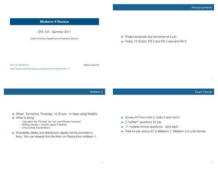
Announcements Midterm II Review STA 104 - Summer 2017 Project proposal due tomorrow at 2 pm Duke University, Department of Statistical Science Friday 12.30 pm, PS 5 and PA 5 due and RA 6 Prof. van den Boom Slides posted at
Announcements Midterm II Review STA 104 - Summer 2017 ▶ Project proposal due tomorrow at 2 pm Duke University, Department of Statistical Science ▶ Friday 12.30 pm, PS 5 and PA 5 due and RA 6 Prof. van den Boom Slides posted at http://www2.stat.duke.edu/courses/Summer17/sta104.001-1/ 1 Midterm 2 Exam Format ▶ When: Tomorrow, Thursday, 12.30 pm - In class using WebEx ▶ Covers HT from Unit 3, Units 4 and Unit 5 ▶ What to bring: – Calculator (No Phones! You can use RStudio however) ▶ 2 “written” questions 22 pts – Writing utensils + scratch paper if desired ▶ 11 multiple choice questions - 2pts each – Cheat sheet (handwritten) ▶ Total 44 pts versus 67 in Midterm 1: Midterm 2 is a bit shorter ▶ Probability tables and distribution applet will be provided in links. You can already find the links on Piazza from midterm 1. 2 3
Unit 4.1 - Inference for Numerical Variables ▶ Two mean testing problems What should you know? – Independent means – Paired (dependent) means ▶ Conditions – Independence – Skew or Approximate Normality 4 5 All other details of the inferential framework is the same... Clicker question HT : test statistic = point estimate − null A study examining the relationship between weights of school SE children and absences found a 95% confidence interval for the difference between the average number of days missed by CI : point estimate ± critical value × SE overweight and normal weight children ( µ overweight − µ normal ) to be 1.3 days to 2.8 days. According to this interval, we are 95% confident that overweight children on average miss Independent means: One mean: Paired means: df = min ( n 1 − 1 , n 2 − 1) df = n − 1 df = n diff − 1 1. 1.3 days fewer to 2.8 days more HT: HT: HT: 2. 1.3 to 2.8 days more H 0 : µ 1 − µ 2 = 0 H 0 : µ = µ 0 H 0 : µ diff = 0 3. 1.3 to 2.8 days fewer x 1 − ¯ x 2 T df = ¯ x − µ x diff − 0 T df = ¯ T df = ¯ sdiff √ s s 2 s 2 4. 1.3 days more to 2.8 days fewer √ n 1 2 √ ndiff n 1 + n 2 CI: CI: than children with normal weight. CI: s s diff x ± t ⋆ x diff ± t ⋆ √ ¯ ¯ s 2 n 1 + s 2 x 1 − ¯ x 2 ± t ⋆ √ n √ n diff ¯ df df 1 2 df n 2 6 7
Unit 4.2 - Bootstrapping Bootstrap interval, standard error ▶ Bootstrapping works as follows: For a random sample of 20 Horror movies, the dot plot below (1) take a bootstrap sample - a random sample taken with replacement shows the distribution of 100 bootstrap medians of the Rotten from the original sample, of the same size as the original sample Tomatoes audience scores. The median of the original sample is (2) calculate the bootstrap statistic - a statistic such as mean, median, 43.5 and the bootstrap standard error is 4.88. Estimate the 90% proportion, etc. computed on the bootstrap samples (3) repeat steps (1) and (2) many times to create a bootstrap distribution - a bootstrap confidence interval for the median RT score of horror distribution of bootstrap statistics movies using the standard error method. ▶ The XX% bootstrap confidence interval can be estimated by ● – the cutoff values for the middle XX% of the bootstrap distribution, ● ● ● ● ● ● ● ● ● ● ● ● ● ● ● ● ● ● ● ● ● ● ● ● ● ● ● ● ● OR ● ● ● ● ● ● ● ● ● ● ● ● ● ● ● ● ● ● ● ● ● ● ● ● ● ● ● ● ● ● ● ● ● ● ● ● ● ● ● ● ● ● ● ● ● ● ● ● ● ● ● ● ● ● ● ● ● ● ● ● ● ● ● ● ●● ● ● ● ● – point estimate ± t ⋆ SE boot 30 35 40 45 50 55 bootstrap medians 8 9 Unit 4.3: Power Unit 4.4: Analysis of VAriance (ANOVA) Decision fail to reject H 0 reject H 0 H 0 true Type 1 Error, α 1 − α ▶ ANOVA tests for some difference in means of many different Truth groups H A true Type 2 Error, β Power, 1 − β ▶ Conditions 1. Independence : ▶ Type 1 error is rejecting H 0 when you shouldn’t have, and the (a) within group: sampled observations must be independent, i.e., probability of doing so is α (significance level) random sampling + 10% rule ▶ Type 2 error is failing to reject H 0 when you should have, and (b) between group: groups must be independent of each other 2. Approximate normality : distribution should be nearly normal within each the probability of doing so is β (a little more complicated to group (if only given summary statistics, think of natural boundaries) calculate) 3. Equal variance : groups should have roughly equal variability ▶ Power of a test is the probability of correctly rejecting H 0 , and the probability of doing so is 1 − β ▶ In hypothesis testing, we want to keep α and β low, but there are inherent trade-offs. 10 11
ANOVA tests for some difference in means of many different groups Null hypothesis: F -statistic: F = SSG / ( k − 1) MSG = H 0 : µ placebo = µ purple = µ brown = . . . = µ peach = µ orange . SSE / ( n − k ) MSE k : # of groups; n : # of obs. Clicker question Df Sum Sq Mean Sq F value Pr( > F) Which of the following is a correct statement of the alternative Between groups k − 1 SSG MSG F obs p obs hypothesis? Within groups n − k SSE MSE Total n − 1 SSG+SSE (a) For any two groups, including the placebo group, no two group means are the same. Note: F distribution is defined by two dfs: df G = k − 1 and (b) For any two groups, not including the placebo group, no two df E = n − k group means are the same. The p-value will be given on exam, compare with the (c) Amongst the jelly bean groups, there are at least two groups that standard α level. have different group means from each other. (d) Amongst all groups, there are at least two groups that have different group means from each other. 12 13 To identify which means are different, use t-tests and the Bonferroni correction To identify which means are different, use t-tests and the Bonferroni correction ▶ If the ANOVA yields a significant results, next natural question is: “Which means are different?” ▶ Use t-tests comparing each pair of means to each other, You will not be asked to perform the actual tests, but you – with a common variance ( MSE from the ANOVA table) instead of each should know: group’s variances in the calculation of the standard error, ▶ How to compute the adjusted Bonferonni significance level α ∗ . – and with a common degrees of freedom ( df E from the ANOVA table) ▶ How to compute the standard error for this test. ▶ Compare resulting p-values to a modified significance level ▶ The associated degrees of freedom for the test statistic. α ⋆ = α K where K = k ( k − 1) is the total number of pairwise tests 2 14 15
Unit 4.4: ANOVA Unit 4.4: ANOVA Application Exercise 4.4 Application Exercise 4.4 Df Sum Sq Mean Sq F p- Df Sum Sq Mean Sq F p- value value Rank 2 1.59 0.795 2.74 0.066 Rank 2 1.59 0.795 2.74 0.066 Residuals 460 135.07 0.29 Residuals 460 135.07 0.29 Total 462 136.66 Total 462 136.66 What significance level should be used for a pair-wise post What is the interpretation of SSG, SSE, and SST in this hoc test comparing the evaluation scores of teaching context? professors and tenured professors? 16 17 Unit 5.1: Inference for a Single Proportion Unit 5.1: Inference for a Single Proportion Distribution of ˆ p Central limit theorem for proportions: Sample proportions will be HT vs. CI for a proportion nearly normally distributed with mean equal to the population mean, ▶ Success-failure condition: √ p (1 − p ) p , and standard error equal to . – CI: At least 10 observed successes and failures n – HT: At least 10 expected successes and failures, calculated using the null value ( ) √ p (1 − p ) p ∼ N mean = p , SE = ˆ ▶ Standard error: n √ p (1 − ˆ p ) – CI: calculate using observed sample proportion: SE = ˆ n √ Conditions: p 0 (1 − p 0 ) – HT: calculate using the null value: SE = n ▶ Independence: Random sample/assignment + 10% rule ▶ At least 10 successes and failures 18 19
Recommend
More recommend
Explore More Topics
Stay informed with curated content and fresh updates.
