Methods for Analyzing ChIP-Seq data Introduction to the ChIP-Seq - PDF document

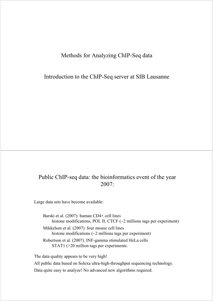
Methods for Analyzing ChIP-Seq data Introduction to the ChIP-Seq server at SIB Lausanne Public ChIP-seq data: the bioinformatics event of the year 2007: Large data sets have become available: Barski et al. (2007): human CD4+ cell lines histone modifications, POL II, CTCF (~2 millions tags per experiment) Mikkelsen et al. (2007): four mouse cell lines histone modifications (~2 millions tags per experiment) Robertson et al. (2007). INF-gamma stimulated HeLa cells STAT1 (>20 million tags per experiments. The data quality appears to be very high! All public data based on Solexa ultra-high-throughput sequencing technology. Data quite easy to analyze! No advanced new algorithms required.

Nature of ChIP-Seq data Short tag sequences of about 30 bp. Sequence correspond to 5’ and 3’ ends of ChIP-fragments DNA fragments have characteristic length resulting from sonication nuclease treatment Tags have some error rates (quality scores available) Not all tags can be uniquely mapped to the genome because of Recent repetitive elements SNPs and other types of genetic variations Tandem repeats (satellite DNA) What can we do with ChIP-seq data: 1. Viewing the data in a genome browser environment: Interesting to virtually every biologist Methods, upload of BED or WIG files 2. Statistical analysis of count distribution over the genome: Example: correlation plot 3. Data reduction and interpretation Partitioning: finding segments of signal-rich and signal-poor region. Peak recognition: Finding peaks of predefined size. 4. Higher-level (downstream) analysis: Example: Finding sequence motifs in peak regions

Data flow in ChIP-Seq data analysis Level 1: Image files (hundreds of Gbytes) Level 2: Tag sequences with quality scores Level 3: Unsorted mapped sequence tag Level 4: Genomic count distribution file (sga, gff, wig format) Level 5: Set of peaks or chromosomal regions (1000 − 10000 lines) The ChIP-Seq Server Purpose: • to make useful data analysis methods available via web interfaces • to provide access to public data sets in useful formats Leading principles • Simple and robust algorithms • Efficient implementations (C programs when necessary) • Generic design: Application not restricted to ChIP-Seq data Interfaces: • Genome browsers • Signal Search Analysis Current implementation status: Under construction!

Application ChIP-Cor Input: • genomic tag count distributions for two features (reference, target) • features may be + and − strand tags from same experiments • applicable to other types of features, e.g. TSS positions Output: • a count correlation histogram • computes number of tag pairs that fall into a distance range. • different normalization options: • count density of target feature • global → relative target feature count density Purpose: • identification of average fragment size • reveals length distribution of enriched domains • provides clues for choosing parameters for peak and partitioning algorithms

Correlation plot: Example 1 Ref: CTCF 5’ tags Target: CTCF 3’ tags Observation: Peak at pos ~75 Count density at peak position: 0.06 Correlation plot: Example 2 Top: Auto-correlation plot of K3K36me3 in mouse ES cells Bottom: Auto-correlation plot of K3K4me3 in mouse ES cells Observations: K3K36me3 → long range correlation K3K36me3 → short range correlation

Application ChIP-Center Input: • Oriented tag counts for a Chip-Seq features Output: • centered, un-oriented tag counts • WIG files for viewing data in a genome browser environment Motivation: • 5’ and 3’ tag position show relative displacement to each other • best estimates for protein-binding site position: 5’ end position + ½ fragment length or 3’ end position − ½ fragment length • centered tag count distribution more useful as input for peak recognition and partitioning algorithms Input page for ChIP-center application Text

Application ChIP-peak Input: • Centered tag counts Output: • List of peak center positions (sga or fps format) Method: • consider only positions which have at least one tag count. • for each positions, determine cumulative tag count in window of width w. • select as peak those positions, which • have cumulative tag count ≥ threshold t. • are local maximum with range ± r. Special server options: • Download of sequences around peak center positions Application ChIP-partition Input: • Centered tag counts Output: • List of signal-enriched regions (beginning, end) Principle: • Optimization of a partition scoring function by a fast dynamic programming algorithm Scoring functions: • Some of scores of signal-rich, signal-poor regions minus a constant penalty for each transition • Score for signal-rich region: length × ( count-density − threshold ) • Score for signal-rich region: length × ( threshold − count-density ) Output options: BED file for genome browser

Application ChIP-part: Results page Viewing the results of the partitoning program in the genome browser Custom tracks: Mikkelsen07: results of ChIP-partition program (BED file) ESHyb.K36: from: http://www.isrec.isb-sib.ch/WIG/HSM07_ESHyb.K36_m_chr12.wig