
SLIDE 1
Sets 1
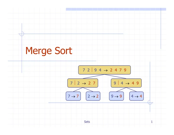
Merge Sort
7 2 ⏐ 9 4 → 2 4 7 9 7 ⏐ 2 → 2 7 9 ⏐ 4 → 4 9 7 → 7 2 → 2 9 → 9 4 → 4
Merge Sort 7 2 9 4 2 4 7 9 7 2 2 7 9 4 4 9 7 7 2 2 9 - - PowerPoint PPT Presentation
Merge Sort 7 2 9 4 2 4 7 9 7 2 2 7 9 4 4 9 7 7 2 2 9 9 4 4 Sets 1 Outline and Reading Divide-and-conquer paradigm (10.1.1) Merge-sort (10.1) Algorithm Merging two sorted sequences
Sets 1
7 2 ⏐ 9 4 → 2 4 7 9 7 ⏐ 2 → 2 7 9 ⏐ 4 → 4 9 7 → 7 2 → 2 9 → 9 4 → 4
Sets 2
Algorithm Merging two sorted sequences Merge-sort tree Execution example Analysis
Sets 3
Divide-and conquer is a general algorithm design paradigm:
Divide: divide the input data
S in two disjoint subsets S1 and S2
Recur: solve the
subproblems associated with S1 and S2
Conquer: combine the
solutions for S1 and S2 into a solution for S
The base case for the recursion are subproblems of size 0 or 1 Merge-sort is a sorting algorithm based on the divide-and-conquer paradigm Like heap-sort
It uses a comparator It has O(n log n) running
time
Unlike heap-sort
It does not use an
auxiliary priority queue
It accesses data in a
sequential manner (suitable to sort data on a disk)
Sets 4
Divide: partition S into
two sequences S1 and S2
each
Recur: recursively sort S1
and S2
Conquer: merge S1 and
S2 into a unique sorted sequence Algorithm mergeSort(S, C) Input sequence S with n elements, comparator C Output sequence S sorted according to C if S.size() > 1 (S1, S2) ← partition(S, n/2) mergeSort(S1, C) mergeSort(S2, C) S ← merge(S1, S2)
Sets 5
The conquer step of merge-sort consists
sorted sequences A and B into a sorted sequence S containing the union
and B Merging two sorted sequences, each with n/2 elements and implemented by means of a doubly linked list, takes O(n) time
Algorithm merge(A, B) Input sequences A and B with n/2 elements each Output sorted sequence of A ∪ B S ← empty sequence while ¬A.isEmpty() ∧ ¬B.isEmpty() if A.first().element() < B.first().element() S.insertLast(A.remove(A.first())) else S.insertLast(B.remove(B.first())) while ¬A.isEmpty() S.insertLast(A.remove(A.first())) while ¬B.isEmpty() S.insertLast(B.remove(B.first())) return S
Sets 6
each node represents a recursive call of merge-sort and stores
unsorted sequence before the execution and its partition sorted sequence at the end of the execution
the root is the initial call the leaves are calls on subsequences of size 0 or 1
Sets 7
7 2 9 4 → 2 4 7 9 3 8 6 1 → 1 3 8 6 7 2 → 2 7 9 4 → 4 9 3 8 → 3 8 6 1 → 1 6 7 → 7 2 → 2 9 → 9 4 → 4 3 → 3 8 → 8 6 → 6 1 → 1 7 2 9 4 ⏐ 3 8 6 1 → 1 2 3 4 6 7 8 9
Sets 8
7 2 ⏐ 9 4 → 2 4 7 9 3 8 6 1 → 1 3 8 6 7 2 → 2 7 9 4 → 4 9 3 8 → 3 8 6 1 → 1 6 7 → 7 2 → 2 9 → 9 4 → 4 3 → 3 8 → 8 6 → 6 1 → 1 7 2 9 4 ⏐ 3 8 6 1 → 1 2 3 4 6 7 8 9
Sets 9
7 2 ⏐ 9 4 → 2 4 7 9 3 8 6 1 → 1 3 8 6 7 ⏐ 2 → 2 7 9 4 → 4 9 3 8 → 3 8 6 1 → 1 6 7 → 7 2 → 2 9 → 9 4 → 4 3 → 3 8 → 8 6 → 6 1 → 1 7 2 9 4 ⏐ 3 8 6 1 → 1 2 3 4 6 7 8 9
Sets 10
7 2 ⏐ 9 4 → 2 4 7 9 3 8 6 1 → 1 3 8 6 7 ⏐ 2 → 2 7 9 4 → 4 9 3 8 → 3 8 6 1 → 1 6 7 → 7 2 → 2 9 → 9 4 → 4 3 → 3 8 → 8 6 → 6 1 → 1 7 2 9 4 ⏐ 3 8 6 1 → 1 2 3 4 6 7 8 9
Sets 11
7 2 ⏐ 9 4 → 2 4 7 9 3 8 6 1 → 1 3 8 6 7 ⏐ 2 → 2 7 9 4 → 4 9 3 8 → 3 8 6 1 → 1 6 7 → 7 2 → 2 9 → 9 4 → 4 3 → 3 8 → 8 6 → 6 1 → 1 7 2 9 4 ⏐ 3 8 6 1 → 1 2 3 4 6 7 8 9
Sets 12
7 2 ⏐ 9 4 → 2 4 7 9 3 8 6 1 → 1 3 8 6 7 ⏐ 2 → 2 7 9 4 → 4 9 3 8 → 3 8 6 1 → 1 6 7 → 7 2 → 2 9 → 9 4 → 4 3 → 3 8 → 8 6 → 6 1 → 1 7 2 9 4 ⏐ 3 8 6 1 → 1 2 3 4 6 7 8 9
Sets 13
7 2 ⏐ 9 4 → 2 4 7 9 3 8 6 1 → 1 3 8 6 7 ⏐ 2 → 2 7 9 4 → 4 9 3 8 → 3 8 6 1 → 1 6 7 → 7 2 → 2 3 → 3 8 → 8 6 → 6 1 → 1 7 2 9 4 ⏐ 3 8 6 1 → 1 2 3 4 6 7 8 9 9 → 9 4 → 4
Sets 14
7 2 ⏐ 9 4 → 2 4 7 9 3 8 6 1 → 1 3 8 6 7 ⏐ 2 → 2 7 9 4 → 4 9 3 8 → 3 8 6 1 → 1 6 7 → 7 2 → 2 9 → 9 4 → 4 3 → 3 8 → 8 6 → 6 1 → 1 7 2 9 4 ⏐ 3 8 6 1 → 1 2 3 4 6 7 8 9
Sets 15
7 2 ⏐ 9 4 → 2 4 7 9 3 8 6 1 → 1 3 6 8 7 ⏐ 2 → 2 7 9 4 → 4 9 3 8 → 3 8 6 1 → 1 6 7 → 7 2 → 2 9 → 9 4 → 4 3 → 3 8 → 8 6 → 6 1 → 1 7 2 9 4 ⏐ 3 8 6 1 → 1 2 3 4 6 7 8 9
Sets 16
7 2 ⏐ 9 4 → 2 4 7 9 3 8 6 1 → 1 3 6 8 7 ⏐ 2 → 2 7 9 4 → 4 9 3 8 → 3 8 6 1 → 1 6 7 → 7 2 → 2 9 → 9 4 → 4 3 → 3 8 → 8 6 → 6 1 → 1 7 2 9 4 ⏐ 3 8 6 1 → 1 2 3 4 6 7 8 9
Sets 17
The height h of the merge-sort tree is O(log n)
at each recursive call we divide in half the sequence,
The overall amount or work done at the nodes of depth i is O(n)
we partition and merge 2i sequences of size n/2i we make 2i+1 recursive calls
Thus, the total running time of merge-sort is O(n log n)
size #seqs depth … … … n/2i 2i i n/2 2 1 n 1
Sets 18
fast sequential data access for huge data sets (> 1M)
fast in-place for large data sets (1K — 1M)
slow in-place for small data sets (< 1K) slow in-place for small data sets (< 1K)
Sets 19
Sets 20
∅
Nodes storing set elements in order Set elements
Sets 21
Generalized merge
A and B Template method genericMerge Auxiliary methods
aIsLess bIsLess bothEqual
Runs in O(nA + nB) time provided the auxiliary methods run in O(1) time
Algorithm genericMerge(A, B) S ← empty sequence while ¬A.isEmpty() ∧ ¬B.isEmpty() a ← A.first().element(); b ← B.first().element() if a < b aIsLess(a, S); A.remove(A.first()) else if b < a bIsLess(b, S); B.remove(B.first()) else { b = a } bothEqual(a, b, S) A.remove(A.first()); B.remove(B.first()) while ¬A.isEmpty() aIsLess(a, S); A.remove(A.first()) while ¬B.isEmpty() bIsLess(b, S); B.remove(B.first()) return S
Sets 22
For intersection: only copy elements that
For union: copy every element from both
Sets 23
We represent a set by the sorted sequence of its elements By specializing the auxliliary methods he generic merge algorithm can be used to perform basic set
union intersection subtraction
The running time of an
should be at most O(nA + nB) Set union:
aIsLess(a, S)
S.insertFirst(a)
bIsLess(b, S)
S.insertLast(b)
bothAreEqual(a, b, S)
Set intersection:
aIsLess(a, S)
{ do nothing }
bIsLess(b, S)
{ do nothing }
bothAreEqual(a, b, S)
Sets 24
7 4 9 6 2 → 2 4 6 7 9 4 2 → 2 4 7 9 → 7 9 2 → 2 9 → 9
Sets 25
Algorithm Partition step Quick-sort tree Execution example
Sets 26
Divide: pick a random
element x (called pivot) and partition S into
L elements less than x E elements equal x G elements greater than x
Recur: sort L and G Conquer: join L, E and G
x x L G E x
Sets 27
We partition an input sequence as follows:
We remove, in turn, each
element y from S and
We insert y into L, E or G,
depending on the result of the comparison with the pivot x
Each insertion and removal is at the beginning or at the end of a sequence, and hence takes O(1) time Thus, the partition step of quick-sort takes O(n) time
Algorithm partition(S, p) Input sequence S, position p of pivot Output subsequences L, E, G of the elements of S less than, equal to,
L, E, G ← empty sequences x ← S.remove(p) while ¬S.isEmpty() y ← S.remove(S.first()) if y < x L.insertLast(y) else if y = x E.insertLast(y) else { y > x } G.insertLast(y) return L, E, G
Sets 28
Each node represents a recursive call of quick-sort and stores
Unsorted sequence before the execution and its pivot Sorted sequence at the end of the execution
The root is the initial call The leaves are calls on subsequences of size 0 or 1
Sets 29
7 2 9 4 → 2 4 7 9 2 → 2 7 2 9 4 3 7 6 1 → 1 2 3 4 6 7 8 9 3 8 6 1 → 1 3 8 6 3 → 3 8 → 8 9 4 → 4 9 9 → 9 4 → 4
Sets 30
2 4 3 1 → 2 4 7 9 9 4 → 4 9 9 → 9 4 → 4 7 2 9 4 3 7 6 1 → 1 2 3 4 6 7 8 9 3 8 6 1 → 1 3 8 6 3 → 3 8 → 8 2 → 2
Sets 31
2 4 3 1 →→ 2 4 7 1 → 1 9 4 → 4 9 9 → 9 4 → 4 7 2 9 4 3 7 6 1 → → 1 2 3 4 6 7 8 9 3 8 6 1 → 1 3 8 6 3 → 3 8 → 8
Sets 32
3 8 6 1 → 1 3 8 6 3 → 3 8 → 8 7 2 9 4 3 7 6 1 → 1 2 3 4 6 7 8 9 2 4 3 1 → 1 2 3 4 1 → 1 4 3 → 3 4 9 → 9 4 → 4
Sets 33
7 9 7 1 → 1 3 8 6 8 → 8 7 2 9 4 3 7 6 1 → 1 2 3 4 6 7 8 9 2 4 3 1 → 1 2 3 4 1 → 1 4 3 → 3 4 9 → 9 4 → 4 9 → 9
Sets 34
7 9 7 1 → 1 3 8 6 8 → 8 7 2 9 4 3 7 6 1 → 1 2 3 4 6 7 8 9 2 4 3 1 → 1 2 3 4 1 → 1 4 3 → 3 4 9 → 9 4 → 4 9 → 9
Sets 35
7 9 7 → 17 7 9 8 → 8 7 2 9 4 3 7 6 1 → 1 2 3 4 6 7 7 9 2 4 3 1 → 1 2 3 4 1 → 1 4 3 → 3 4 9 → 9 4 → 4 9 → 9
Sets 36
The worst case for quick-sort occurs when the pivot is the unique minimum or maximum element One of L and G has size n − 1 and the other has size 0 The running time is proportional to the sum n + (n − 1) + … + 2 + 1 Thus, the worst-case running time of quick-sort is O(n2)
time depth 1 n − 1 … … n − 1 1 n
Sets 37
Consider a recursive call of quick-sort on a sequence of size s
Good call: the sizes of L and G are each less than 3s/4 Bad call: one of L and G has size greater than 3s/4
A call is good with probability 1/2
1/2 of the possible pivots cause good calls:
7 9 7 1 → 1 7 2 9 4 3 7 6 1 9 2 4 3 1 7 2 9 4 3 7 6 1 7 2 9 4 3 7 6 1
Good call Bad call 1 2 3 4 5 6 7 8 9 10 11 12 13 14 15 16 Good pivots Bad pivots Bad pivots
Sets 38
Probabilistic Fact: The expected number of coin tosses required in
For a node of depth i, we expect
i/2 ancestors are good calls The size of the input sequence for the current call is at most (3/4)i/2n
s(r) s(a) s(b) s(c) s(d) s(f) s(e) time per level expected height O(log n) O(n) O(n) O(n) total expected time: O(n log n)
Therefore, we have
For a node of depth 2log4/3n,
the expected input size is one
The expected height of the
quick-sort tree is O(log n)
The amount or work done at the nodes of the same depth is O(n) Thus, the expected running time
Sets 39
Quick-sort can be implemented to run in-place In the partition step, we use replace operations to rearrange the elements of the input sequence such that
the elements less than the
pivot have rank less than h
the elements equal to the pivot
have rank between h and k
the elements greater than the
pivot have rank greater than k
The recursive calls consider
elements with rank less than h elements with rank greater
than k Algorithm inPlaceQuickSort(S, l, r) Input sequence S, ranks l and r Output sequence S with the elements of rank between l and r rearranged in increasing order if l ≥ r return i ← a random integer between l and r x ← S.elemAtRank(i) (h, k) ← inPlacePartition(x) inPlaceQuickSort(S, l, h − 1) inPlaceQuickSort(S, k + 1, r)
Sets 40
Scan j to the right until finding an element > x. Scan k to the left until finding an element < x. Swap elements at indices j and k
3 2 5 1 0 7 3 5 9 2 7 9 8 9 7 6 9
3 2 5 1 0 7 3 5 9 2 7 9 8 9 7 6 9
Sets 41
in-place, randomized fastest (good for large inputs)
sequential data access fast (good for huge inputs)
in-place fast (good for large inputs)
in-place slow (good for small inputs) in-place slow (good for small inputs)
Sets 42
1 2 3 4 5 6 7 8 9 B 1, c 7, d 7, g 3, b 3, a 7, e ∅ ∅ ∅ ∅ ∅ ∅ ∅
Sets 43
Let be S be a sequence of n (key, element) items with keys in the range [0, N − 1] Bucket-sort uses the keys as indices into an auxiliary array B
Phase 1: Empty sequence S by moving each item (k, o) into its bucket B[k] Phase 2: For i = 0, …, N − 1, move the items of bucket B[i] to the end of sequence S
Analysis:
Phase 1 takes O(n) time Phase 2 takes O(n + N) time
Bucket-sort takes O(n + N) time
Algorithm bucketSort(S, N) Input sequence S of (key, element) items with keys in the range [0, N − 1] Output sequence S sorted by increasing keys B ← array of N empty sequences while ¬S.isEmpty() f ← S.first() (k, o) ← S.remove(f) B[k].insertLast((k, o)) for i ← 0 to N − 1 while ¬B[i].isEmpty() f ← B[i].first() (k, o) ← B[i].remove(f) S.insertLast((k, o))
Sets 44
1 2 3 4 5 6 7 8 9
∅ ∅ ∅ ∅ ∅ ∅ ∅
Sets 45
The keys are used as
indices into an array and cannot be arbitrary
No external comparator
The relative order of
any two items with the same key is preserved after the execution of the algorithm
Integer keys in the range [a, b]
Put item (k, o) into bucket
B[k − a]
String keys from a set D of
possible strings, where D has constant size (e.g., names of the 50 U.S. states)
Sort D and compute the rank
r(k) of each string k of D in the sorted sequence
Put item (k, o) into bucket
B[r(k)]
Sets 46
The Cartesian coordinates of a point in space are a 3-tuple
(x1, x2, …, xd) < (y1, y2, …, yd)
x1 < y1 ∨ x1 = y1 ∧ (x2, …, xd) < (y2, …, yd)
Sets 47
Let Ci be the comparator that compares two tuples by their i-th dimension Let stableSort(S, C) be a stable sorting algorithm that uses comparator C Lexicographic-sort sorts a sequence of d-tuples in lexicographic order by executing d times algorithm stableSort, one per dimension Lexicographic-sort runs in O(dT(n)) time, where T(n) is the running time of stableSort Algorithm lexicographicSort(S) Input sequence S of d-tuples Output sequence S sorted in lexicographic order for i ← d downto 1 stableSort(S, Ci)
(7,4,6) (5,1,5) (2,4,6) (2, 1, 4) (3, 2, 4) (2, 1, 4) (3, 2, 4) (5,1,5) (7,4,6) (2,4,6) (2, 1, 4) (5,1,5) (3, 2, 4) (7,4,6) (2,4,6) (2, 1, 4) (2,4,6) (3, 2, 4) (5,1,5) (7,4,6)
Sets 48
Radix-sort is a specialization of lexicographic-sort that uses bucket-sort as the stable sorting algorithm in each dimension Radix-sort is applicable to tuples where the keys in each dimension i are integers in the range [0, N − 1] Radix-sort runs in time O(d( n + N)) Algorithm radixSort(S, N) Input sequence S of d-tuples such that (0, …, 0) ≤ (x1, …, xd) and (x1, …, xd) ≤ (N − 1, …, N − 1) for each tuple (x1, …, xd) in S Output sequence S sorted in lexicographic order for i ← d downto 1 bucketSort(S, N)
Sets 49
Algorithm binaryRadixSort(S) Input sequence S of b-bit integers Output sequence S sorted replace each element x
for i ← 0 to b − 1 replace the key k of each item (k, x) of S with bit xi of x bucketSort(S, 2)
Sets 50
Sets 51
Sets 52
They sort by making comparisons between pairs of objects Examples: bubble-sort, selection-sort, insertion-sort, heap-sort,
merge-sort, quick-sort, ...
Is xi < xj? yes no
Sets 53
xi < xj ? xa < xb ? xm < xo ? xp < xq ? xe < xf ? xk < xl ? xc < xd ?
Sets 54
The height of this decision tree is a lower bound on the running time Every possible input permutation must lead to a separate leaf
If not, some input …4…5… would have same output ordering as
…5…4…, which would be wrong. Since there are n!=1*2*…*n leaves, the height is at least log (n!)
minimum height (time) log (n!) xi < xj ? xa < xb ? xm < xo ? xp < xq ? xe < xf ? xk < xl ? xc < xd ? n!
Sets 55
2
n
Sets 56
Sets 57
Sets 58
Prune: pick a random element x
(called pivot) and partition S into
L elements less than x E elements equal x G elements greater than x
Search: depending on k, either
answer is in E, or we need to recur on either L or G x x L G E
Sets 59
We partition an input sequence as in the quick-sort algorithm:
We remove, in turn, each
element y from S and
We insert y into L, E or G,
depending on the result of the comparison with the pivot x
Each insertion and removal is at the beginning or at the end of a sequence, and hence takes O(1) time Thus, the partition step of quick-select takes O(n) time
Algorithm partition(S, p) Input sequence S, position p of pivot Output subsequences L, E, G of the elements of S less than, equal to,
L, E, G ← empty sequences x ← S.remove(p) while ¬S.isEmpty() y ← S.remove(S.first()) if y < x L.insertLast(y) else if y = x E.insertLast(y) else { y > x } G.insertLast(y) return L, E, G
Sets 60
Each node represents a recursive call of quick-select, and
stores k and the remaining sequence
Sets 61
Consider a recursive call of quick-select on a sequence of size s
Good call: the sizes of L and G are each less than 3s/4 Bad call: one of L and G has size greater than 3s/4
A call is good with probability 1/2
1/2 of the possible pivots cause good calls:
7 9 7 1 → 1 7 2 9 4 3 7 6 1 9 2 4 3 1 7 2 9 4 3 7 6 1 7 2 9 4 3 7 6 1
Good call Bad call 1 2 3 4 5 6 7 8 9 10 11 12 13 14 15 16 Good pivots Bad pivots Bad pivots
Sets 62
Probabilistic Fact #1: The expected number of coin tosses required in
Probabilistic Fact #2: Expectation is a linear function:
E(X + Y ) = E(X ) + E(Y ) E(cX ) = cE(X )
Let T(n) denote the expected running time of quick-select. By Fact #2,
T(n) < T(3n/4) + bn*(expected # of calls before a good call)
By Fact #1,
T(n) < T(3n/4) + 2bn
That is, T(n) is a geometric series:
T(n) < 2bn + 2b(3/4)n + 2b(3/4)2n + 2b(3/4)3n + …
So T(n) is O(n).
Sets 63
We can do selection in O(n) worst-case time. Main idea: recursively use the selection algorithm itself to find a good pivot for quick-select:
Divide S into n/5 sets of 5 each Find a median in each set Recursively find the median of the “baby” medians.
See Exercise C-4.24 for details of analysis.
1 2 3 4 5 1 2 3 4 5 1 2 3 4 5 1 2 3 4 5 1 2 3 4 5 1 2 3 4 5 1 2 3 4 5 1 2 3 4 5 1 2 3 4 5 1 2 3 4 5 1 2 3 4 5
Sets 64
log 1 log log log log
+ + −
ε ε
a k a k a a a
b b b b b