Medical Imaging with Deep Learning PathologyGAN: Learning deep - PowerPoint PPT Presentation
Medical Imaging with Deep Learning PathologyGAN: Learning deep representations of cancer tissue Adalberto Claudio Quiros a.claudio-quiros.1@research.gla.ac.uk Roderick Murray-Smith roderick.murray-smith@glasgow.ac.uk Ke Yuan
Medical Imaging with Deep Learning PathologyGAN: Learning deep representations of cancer tissue Adalberto Claudio Quiros a.claudio-quiros.1@research.gla.ac.uk Roderick Murray-Smith roderick.murray-smith@glasgow.ac.uk Ke Yuan ke.yuan@glasgow.ac.uk University of Glasgow, Computing Science Department June 26, 2020
Motivation Cancer and Tissue Imaging ∙ Cancer is a heterogeneous disease, with complex micro-environments where lymphocytes, stromal, and cancer cells interact with the tissue and blood vessels. ∙ Although the genomic and transcriptomic diversity in tumors is quite high, phenotype between/within tumor such as cellular behaviours and tumor micro-environments remains poorly understood. Why generative models? ∙ Limitation of supervised learning: Expensiveness of data collection and labeling, it cannot provide unknown information about the data. ∙ A generative model can to identify and reproduce the difgerent types of tissue. ∙ Disentangled representations can provide further understanding on phenotype diversity between and within tumors. 1
Model We start with BigGAN and Relativistic Average Discriminator. Figure 1: Starting point: BigGAN with Relativistic Average Discriminator. ̃ 𝐸 (𝑦 𝑠 ) = sigmoid (𝐷 (𝑦 𝑠 ) − 𝔽 𝑦 𝑔 ∼ℚ 𝐷 (𝑦 𝑔 ))), ̃ (2) 𝐸 (𝑦 𝑠 ))] , ̃ 2 (1) 𝐸 (𝑦 𝑔 ))] , ̃ fake data, and 𝐷(𝑦) is the non-transformed discriminator output or critic: Equations 2 and 3, where ℙ is the distribution of real data, ℚ is the distribution for the Loss function: The discriminator, and generator loss function are formulated as in 𝑀 𝐸𝑗𝑡 = −𝔽 𝑦 𝑠 ∼ℙ [ log ( ̃ 𝐸 (𝑦 𝑠 ))] − 𝔽 𝑦 𝑔 ∼ℚ [ log (1 − 𝑀 𝐻𝑓𝑜 = −𝔽 𝑦 𝑔 ∼ℚ [ log ( ̃ 𝐸 (𝑦 𝑔 ))] − 𝔽 𝑦 𝑠 ∼ℙ [ log (1 − 𝐸 (𝑦 𝑔 ) = sigmoid (𝐷 (𝑦 𝑔 ) − 𝔽 𝑦 𝑠 ∼ℙ 𝐷 (𝑦 𝑠 )) .
Model High quality tissue image generation. Limitation: No interpretability or structure in the latent space. Figure 2: (a): Images ( 224 × 224 , 448 × 448 ) from PathologyGAN trained on H&E breast cancer tissue. (b): Real images, Inception-V1 closest neighbor to the generated above. 3
Model Motivation: Can we modify or introduce changes so we have an ordered latent space based on cancer tissue characteristics? We introduce two features from StyleGAN [1]: ∙ Mapping Network [ 𝑥 ∼ 𝑁(𝑨) ]: ∙ Neural network that allows to freely optimize the latent space to disentangle high level features in the tissue. ∙ Style Mixing Regularization: ∙ To further enforce localize tissue characteristics in the latent space, we use two difgerent latent vectors ( 𝑨 1 , 𝑨 2 ) to generate a single image. ∙ We can do this since the latent vector is feed at every level of the generator, we randomly choose a layer in the generator and feed each difgerent latent vector to each half. Figure 3: PathologyGAN high level representation 4
Results - Image Quality 2. Cancer tissue characteristics as cancer, lymphocyte, stroma cells count and density: highlighted with a green color, while lymphocytes and stromal cells are highlighted in yellow. Figure 4: CRImage identifies difgerent cell types in our generated images. Cancer cells are density) ∙ Each image is quantified into a vector: (# cancer cells, # lymph. and stroma, cancer cell image. We use an external tool, CRImage, based on SVM to quantify these in the tissue (FID). Fréchet Distance: Wasserstein distance between two Gaussians: 1. Convolutional Features from an pretrained Inception-V1: Fréchet Inception Distance 1/2 ) ; We want to measure difgerences between real and generated tissue distributions. 5 2 + Tr (Σ 𝑠 + Σ − 2 (Σ 𝑠 Σ ) FID = ∥𝜈 𝑠 − 𝜈 ∥ where 𝑌 𝑠 ∼ 𝒪 (𝜈 𝑠 , Σ 𝑠 ) and 𝑌 ∼ 𝒪 (𝜈 , Σ )
Results - Image Quality As a reference, values are similar to ImageNet models of BigGAN [2] and SAGAN [3], with FIDs of 7.4 and 18.65 respectively or StyleGAN [1] trained on FFHQ with FID of 4.40: Model Inception FID CRImage FID PathologyGAN 16.65 ± 2.5 9.86 ± 0.4 Table 1: Evaluation of PathologyGANs. Mean and standard deviations are computed over three difgerent random initializations. The low FID scores in both feature space suggest consistent and accurate representations. 6
Results - Patholigists’ Interpretation Pathologists’ interpretation: Motivation: Test if experts that work with tissue images find artifacts that give away generated tissue. 1. Test I: 25 Sets of 8 images - Pathologists were asked to find the only fake image in each set. 2. Test II: 50 Individual images - Pathologists were asked to rate all individual images from 1 to 5, where 5 meant the image appeared the most real. Figure 5: Example of Test I. Figure 6: Examples of Test II. 7
Results - Patholigists’ Interpretation Pathologists’ interpretation: 1. Test I: Pathologist 1 and 2 were able to find only 2/25 sets and 3/25 fake images. 2. Test II: Figure 7 - The near random classification performance from both expert pathologists suggests that generated tissue images do not present artifacts that give away the tissue as generated. Figure 7: ROC curve of Pathologists’ classification for tissue images. 8
Results - Representation Learning Do we have any kind of structure in the latent space? 1. We generated 10, 000 tissue images, each of them with its associated latent vector 𝑥 ∈ ℝ 200 2. For each tissue image, we run CRImage to get the count of cancer cells in the tissue. 3. We created 9 difgerent buckets for cancer cell counts. Class 0 accounts for images with the lowest count cancer cells, on the other extreme Class 8 accounts for images with the largest counts. 4. We run UMAP[4] to perform dimensionality reduction from 200 dimensions to 2 dimensions over the complete 10, 000 𝑥 lantent vectors. Figure 8: Preprocessing of data for latent space interpreztation. 9
Pathologygan - Representation Learning Properties Difgerence between PathologyGAN’s and BigGAN’s latent space: ∙ (a) PathologyGAN shows structure in the latent space 𝑥 making the image generation interpretable, increasing counts in cancer cells correspond to moving the selected vector from quadrant 𝐽𝑊 to quadrant 𝐽𝐽 ∙ (b) Vector samples are randomly placed in the BigGAN’s latent space 𝑥 . Figure 9: Contrast between PathologyGAN’s latent space (a) and BigGAN’s (b). 10
Results - Representation Learning Figure 10: Scatter plots with 𝑥 latent vectors on PathologyGAN’s latent space. Each sub-figure shows datapoints only related to one of the classes, and each class is subject to the count of cancer cells in the tissue image, (a) [class 0] are associated to images with the lowest number of cancer cells, (h) [class 8] with the largest. 11
Results - Representation Learning Figure 11: Density plots with 𝑥 latent vectors on PathologyGAN’s latent space. Each sub-figure shows datapoints only related to one of the classes, and each class is subject to the count of cancer cells in the tissue image, (a) [class 0] are associated to images with the lowest number of cancer cells, (h) [class 8] with the largest. 12
Results - Representation Learning Linear interpolation: ∙ We captured two latent vectors 𝑨 with associated tissue: benign (less cancer cells, leħt end) and malignant tissue (more cancer cells, right end). ∙ We performed a linear interpolation of 8 stages between these two vectors and fed the generator. Conclusions: ∙ PathologyGAN (a) includes an increasing population of cancer cells rather than a fading efgect from BigGAN (b). ∙ PathologyGAN (a) better translates high level features of the images from the latent space vectors. Figure 12: (a) PathologyGAN model. (b) BigGAN model. 13
Results - Representation Learning Vector Operations: 1. We gather latent vectors 𝑨 that generate images with difgerent high level features: Benign tissue, lymphocytes, stroma, and tumorous tissue. 2. We performed difgerent linear vector operations before we fed the generator. Conclusions: 1. The resulting images hold the feature transformations implied in the vector operations. Figure 13: Examples of vector operations. 14
Acknowledgements Thanks to Joanne Edwards and Elizabeth Mallon for the helpful insight and discussion on digital pathology. ∙ Dr. Joanne Edwards - University of Glasgow ∙ Dr. Elizabeth Mallon - University of Glasgow 15
Thanks Thank you for checking out our work! 16
[1] Tero Karras, Samuli Laine, and Timo Aila. A style-based generator architecture for generative adversarial networks. 2019 IEEE/CVF Conference on Computer Vision and Pattern Recognition (CVPR) , Jun 2019. [2] Andrew Brock, Jefg Donahue, and Karen Simonyan. Large scale gan training for high fidelity natural image synthesis, 2018. [3] Han Zhang, Ian Goodfellow, Dimitris Metaxas, and Augustus Odena. Self-attention generative adversarial networks, 2018. [4] Leland McInnes, John Healy, and James Melville. Umap: Uniform manifold approximation and projection for dimension reduction, 2018. 17
Recommend
More recommend
Explore More Topics
Stay informed with curated content and fresh updates.
