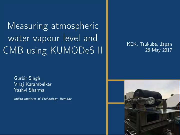
Measuring atmospheric water vapour level and KEK, Tsukuba, Japan - PowerPoint PPT Presentation

Measuring atmospheric water vapour level and KEK, Tsukuba, Japan CMB using KUMODeS II 26 May 2017 Gurbir Singh Viraj Karambelkar Yashvi Sharma Indian Institute of Technology, Bombay

1 Introduction KUMODeS II Theory Model LMFit 2 Observations 3 CMB

Introduction images/IM_logo.pdf Schematic Diagram of KUMODeS II

Introduction images/IM_logo.pdf KUMODeS II Using KUMODeS II, we measured ◮ Precipitable Water Vapour (PWV)

Introduction images/IM_logo.pdf KUMODeS II Using KUMODeS II, we measured ◮ Precipitable Water Vapour (PWV) ◮ Cosmic Microwave Background (CMB)

Introduction images/IM_logo.pdf Theory ◮ Nyquist Theorem P = kGBT

Introduction images/IM_logo.pdf Theory ◮ Nyquist Theorem P = kGBT ◮ Y factor method P hot = kGB ( T noise + 300 ) P cold = kGB ( T noise + 77 )

Introduction images/IM_logo.pdf Theory ◮ Nyquist Theorem P = kGBT ◮ Y factor method P hot = kGB ( T noise + 300 ) P cold = kGB ( T noise + 77 ) ◮ Sky Observation � � P sky = kGB T noise + T sky

Introduction images/IM_logo.pdf Model Used AM to model the atmospheric emission

Introduction images/IM_logo.pdf LMFit AM + mx + c � �� � Oxygen + CMB

Introduction images/IM_logo.pdf LMFit AM + mx + c � �� � Oxygen + CMB ◮ The parameters were PWV, m, and c.

Introduction images/IM_logo.pdf LMFit AM + mx + c � �� � Oxygen + CMB ◮ The parameters were PWV, m, and c. ◮ The data was fit according to this model using LMFit

Observations images/IM_logo.pdf First run The noise temperature observed was

Observations images/IM_logo.pdf Improvement By replacing a cable, we were able to improve the noise temperature. Figure:

Observations images/IM_logo.pdf Improvement By installing an isolator, the noise temperature was further improved. Figure: Block diagram with isolator

Observations images/IM_logo.pdf Improvement Figure: Comparison of noise with and without isolator

Observations images/IM_logo.pdf Sky Observations

Observations images/IM_logo.pdf PWV fit

CMB Measurement

CMB images/IM_logo.pdf CMB Measurement using KUMODeS II setup When the sky is observed using the radio receiver, ◮ 1 P out = kGB ( T noise + T atm × cos ( z ) + T cmb ) z : zenith angle

CMB images/IM_logo.pdf CMB Measurement using KUMODeS II setup When the sky is observed using the radio receiver, ◮ 1 P out = kGB ( T noise + T atm × cos ( z ) + T cmb ) z : zenith angle Also, from the Y-Factor method,

CMB images/IM_logo.pdf CMB Measurement using KUMODeS II setup When the sky is observed using the radio receiver, ◮ 1 P out = kGB ( T noise + T atm × cos ( z ) + T cmb ) z : zenith angle Also, from the Y-Factor method, ◮ P hot = kGB ( T noise + 300 )

CMB images/IM_logo.pdf CMB Measurement using KUMODeS II setup When the sky is observed using the radio receiver, ◮ 1 P out = kGB ( T noise + T atm × cos ( z ) + T cmb ) z : zenith angle Also, from the Y-Factor method, ◮ P hot = kGB ( T noise + 300 ) ◮ 1 P out − P hot = kGB ( T atm × cos ( z ) + T cmb − 300 )

CMB images/IM_logo.pdf CMB Measurement using KUMODeS II setup When the sky is observed using the radio receiver, ◮ 1 P out = kGB ( T noise + T atm × cos ( z ) + T cmb ) z : zenith angle Also, from the Y-Factor method, ◮ P hot = kGB ( T noise + 300 ) ◮ 1 P out − P hot = kGB ( T atm × cos ( z ) + T cmb − 300 ) A plot of (Pout-Phot)/kGB vs sec(z) is a straight line with intercept (T cmb − 300 )

CMB images/IM_logo.pdf Observations Figure: CMB

CMB images/IM_logo.pdf Results We obtained the cmb temperature spectrum as Figure: CMB temperature vs frequency

CMB images/IM_logo.pdf Conclusions The cmb result is off from the expected value of 2.7K This is probably because of the following reasons- ◮ Reflections from the mirror and ground When we plot Tsky vs Frequency, we observe a trend that the sky temperatures increase with time. Also, a standing wave pattern (wavelength 1m approx) is seen in the sky temperatures taken at later times. However, no such increase in temperatures are seen in readings taken inside the building during noise calculations.

CMB images/IM_logo.pdf Conclusions The cmb result is off from the expected value of 2.7K This is probably because of the following reasons- ◮ Reflections from the mirror and ground When we plot Tsky vs Frequency, we observe a trend that the sky temperatures increase with time. Also, a standing wave pattern (wavelength 1m approx) is seen in the sky temperatures taken at later times. However, no such increase in temperatures are seen in readings taken inside the building during noise calculations. Hence, the increase is probably due to reflections from the mirror used to focus the radiation and ground.

CMB images/IM_logo.pdf Conclusions Figure: Sky Temperatures

CMB images/IM_logo.pdf Conclusions

CMB images/IM_logo.pdf Conclusion Uncertainty in gain of Amplifier ◮ We have calibrated the gain of the receiver by taking two Y-Factor measurements, before and after the sky measurements. Then, we used linear extrapolation to find the gain of the amplifier during measurement time.

CMB images/IM_logo.pdf Conclusion Uncertainty in gain of Amplifier ◮ We have calibrated the gain of the receiver by taking two Y-Factor measurements, before and after the sky measurements. Then, we used linear extrapolation to find the gain of the amplifier during measurement time. ◮ However the gain of the amplifier is extremely sensitive to temperature, and the gain profile may not be linear. In other telescopes, and even KUMODeS, real time gain calibration is done using a cold body inside the telescope.

Thank You!