MapReduce and Frequent Itemsets Mining Yang Wang 1 MapReduce - PowerPoint PPT Presentation
MapReduce and Frequent Itemsets Mining Yang Wang 1 MapReduce (Hadoop) Programming model designed for: Large Datasets (HDFS) Large files broken into chunks Chunks are replicated on different nodes Easy Parallelization Takes
MapReduce and Frequent Itemsets Mining Yang Wang 1
MapReduce (Hadoop) Programming model designed for: ● Large Datasets (HDFS) ○ Large files broken into chunks ○ Chunks are replicated on different nodes ● Easy Parallelization ○ Takes care of scheduling ● Fault Tolerance ○ Monitors and re-executes failed tasks
MapReduce 3 Steps ● Map: ○ Apply a user written map function to each input element. ○ The output of Map function is a set of key- value pairs. ● GroupByKey : ○ Sort and Shuffle : Sort all key-value pairs by key and output key-(list of value pairs) ● Reduce ○ User written reduce function applied to each key-[list of value] pairs
Coping with Failure MapReduce is designed to deal with compute nodes failing Output from previous phases is stored. Re- execute failed tasks, not whole jobs. Blocking Property : no output is used until the task is complete. Thus, we can restart a Map task that failed without fear that a Reduce task has already used some output of the failed Map task.
Data Flow Systems ● MapReduce uses two ranks of tasks: ○ One is Map and other is Reduce ○ Data flows from first rank to second rank ● Data Flow Systems generalise this: ○ Allow any number of tasks ○ Allow functions other than Map and Reduce ● Spark is the most popular data-flow system. ○ RDD’s : Collection of records ○ Spread across clusters and read-only.
Frequent Itemsets ● The Market-Basket Model ○ Items ○ Baskets ○ Count how many baskets contain an itemset ○ Support threshold => frequent itemsets ● Application ○ Confidence ■ Pr(D | A, B, C)
Computation Model ● Count frequent pairs ● Main memory is the bottleneck ● How to store pair counts? ○ Triangular matrix/Table ● Frequent pairs -> frequent items ● A-Priori Algorithm ○ Pass 1 - Item counts ○ Pass 2 - Frequent items + pair counts ● PCY ○ Pass 1 - Hash pairs into buckets ■ Infrequent bucket -> infrequent pairs ○ Pass 2 - Bitmap for buckets ■ Count pairs w/ frequent items and frequent bucket
All (Or Most) Frequent Itemsets ● Handle Large Datasets ● Simple Algorithm ○ Sample from all baskets ○ Run A-Priori/PCY in main memory with lower threshold ○ No guarantee ● SON Algorithm ○ Partition baskets into subsets ○ Frequent in the whole => frequent in at least one subset ● Toivonen’s Algorithm ○ Negative Border - not frequent in the sample but all immediate subsets are ○ Pass 2 - Count frequent itemsets and sets in their negative border ○ What guarantee?
Locality Sensitive Hashing and Clustering Hongtao Sun 1 2
Locality-Sensitive Hashing Main idea: ● What: hashing techniques to map similar items to the same bucket → candidate pairs ● Benefits: O(N) instead of O(N 2 ): avoid comparing all pairs of items ○ Downside: false negatives and false positives ● Applications : similar documents, collaborative filtering, etc. For the similar document application, the main steps are: 1.Shingling - converting documents to set representations 2.Minhashing - converting sets to short signatures using random permutations 3.Locality-sensitive hashing - applying the “b bands of r rows” technique on the signature matrix to an “s-shaped” curve
Locality-Sensitive Hashing Shingling: ● Convert documents to set representation using sequences of k tokens ● Example: abcabc with k = 2 shingle size and character tokens → {ab, bc, ca} ● Choose large enough k → lower probability shingle s appears in document ● Similar documents → similar shingles (higher Jaccard similarity) Jaccard Similarity: J(S 1 , S 2 ) = |S 1 ∩ S 2 | / |S 1 ∪ S 2 | Minhashing: ● Creates summary signatures: short integer vectors that represent the sets and reflect their similarity
Locality-Sensitive Hashing General Theory: ● Distance measures d (similar items are “close”): ○ Ex) Euclidean, Jaccard, Cosine, Edit, Hamming ● LSH families: ○ A family of hash functions H is (d 1 , d 2 , p 1 , p 2 )-sensitive if for any x and y: ■ If d(x, y) <= d 1 , Pr [h(x) = h(y)] >= p 1 ; and ■ If d(x, y) >= d 2 , Pr [h(x) = h(y)] <= p 2 . ● Amplification of an LSH families (“bands” technique): ○ AND construction (“rows in a band”) ○ OR construction (“many bands”) ○ AND-OR/OR-AND compositions
Locality-Sensitive Hashing Suppose that two documents have Jaccard similarity s. Step-by-step analysis of the banding technique (b bands of r rows each) ● Probability that signatures agree in all rows of a particular band: ○ s r ● Probability that signatures disagree in at least one row of a particular band: ○ 1 - s r ● Probability that signatures disagree in at least one row of all of the bands: ○ (1 - s r ) b ● Probability that signatures agree in all rows of a particular band ⇒ Become candidate pair: ○ 1 - (1 - s r ) b
Locality-Sensitive Hashing A general strategy for composing families of minhash functions: AND construction (over r rows in a single band): ● (d 1 , d 2 , p 1 , p 2 )-sensitive family ⇒ (d 1 , d 2 , p 1 r , p 2 r )-sensitive family ● Lowers all probabilities OR construction (over b bands ): ● (d 1 , d 2 , p 1 , p 2 )-sensitive family ⇒ (d 1 , d 2 , 1 - (1 - p 1 ) b , 1 - (1 - p 2 ) b )-sensitive family ● Makes all probabilities rise We can try to make p 1 → 1 (lower false negatives) and p 2 → 0 (lower false positives), but this can require many hash functions.
Clustering What : Given a set of points and a distance measure , group them into “ clusters ” so that a point is more similar to other points within the cluster compared to points in other clusters (unsupervised learning - without labels) How : Two types of approaches ● Point assignments ○ Initialize centroids ○ Assign points to clusters, iteratively refine ● Hierarchical : ○ Each point starts in its own cluster ○ Agglomerative: repeatedly combine nearest clusters
Point Assignment Clustering Approaches ● Best for spherical/convex cluster shapes ● k-means: initialize cluster centroids, assign points to the nearest centroid, iteratively refine estimates of the centroids until convergence ○ Euclidean space ○ Sensitive to initialization (K-means++) ○ Good values of “k” empirically derived ○ Assumes dataset can fit in memory ● BFR algorithm: variant of k-means for very large datasets (residing on disk) ○ Keep running statistics of previous memory loads ○ Compute centroid, assign points to clusters in a second pass
Hierarchical Clustering ● Can produce clusters with unusual shapes ○ e.g. concentric ring-shaped clusters ● Agglomerative approach : ○ Start with each point in its own cluster ○ Successively merge two “nearest” clusters until convergence ● Differences from Point Assignment : ○ Location of clusters: centroid in Euclidean spaces, “clustroid” in non-Euclidean spaces ○ Different intercluster distance measures: e.g. merge clusters with smallest max distance (worst case), min distance (best case), or average distance (average case) between points from each cluster ○ Which method works best depends on cluster shapes, often trial and error
Dimensionality Reduction and Recommender Systems Jayadev Bhaskaran 21
Dimensionality Reduction ● Motivation ○ Discover hidden structure ○ Concise description Save storage ■ Faster processing ■ ● Methods ○ SVD M = UΣV T ■ U user-to-concept matrix ● V movie-to-concept matrix ● Σ “strength” of each concept ● ○ CUR Decomposition M = CUR ■
SVD ● M = UΣV T U T U = I, V T V = I, Σ diagonal with non-negative entries ○ Best low-rank approximation (singular value thresholding) ○ Always exists for any real matrix M ○ ● Algorithm Find Σ, V ○ Find eigenpairs of M T M -> (D, V) ■ Σ is square root of eigenvalues D ■ V is the right singular vectors ■ Similarly U can be read off from eigenvectors of MM T ■ Power method: random init + repeated matrix-vector multiply (normalized) gives ○ principal evec Note: Symmetric matrices ○ M T M and MM T are both real, symmetric matrices ■ Real symmetric matrix: eigendecomposition QΛQ T ■
CUR ● M = CUR ● Non-uniform sampling Row/Column importance ○ proportional to norm U: pseudoinverse of ○ submatrix with sampled rows R & columns C ● Compared to SVD Interpretable (actual columns ○ & rows) Sparsity preserved (U,V dense ○ but C,R sparse) May output redundant ○ features
Recommender Systems: Content- Based What: Given a bunch of users, items and ratings, want to predict missing ratings How: Recommend items to customer x similar to previous items rated highly by x ● Content-Based ○ Collect user profile x and item profile i ○ Estimate utility: u( x , i ) = cos( x , i )
Recommender Systems: Collaborative Filtering ● user-user CF vs item-item CF user-user CF: estimate a user’s rating based on ratings of similar users who have rated ○ the item ; similar definition for item-item CF ● Similarity metrics Jaccard similarity: binary ○ Cosine similarity: treats missing ratings as “negative” ○ Pearson correlation coeff: remove mean of non-missing ratings (standardized) ○ ● Prediction of item i from user x: (s xy = sim(x,y)) ● Remove baseline estimate and only model rating deviations from baseline estimate, so that we’re not affected by user/item bias
Recommend
More recommend
Explore More Topics
Stay informed with curated content and fresh updates.
