Machine Translation May 28, 2013 Christian Federmann Saarland - PowerPoint PPT Presentation
Machine Translation May 28, 2013 Christian Federmann Saarland University cfedermann@coli.uni-saarland.de Language Technology II SS 2013 Decoding The decoder uses source sentence f and phrase table to estimate P(e|f) uses LM
Machine Translation May 28, 2013 Christian Federmann Saarland University cfedermann@coli.uni-saarland.de Language Technology II SS 2013
Decoding The decoder … uses source sentence f and phrase table to estimate P(e|f) uses LM to estimate P(e) searches for target sentence e that maximizes P(e)*P(f|e) cfedermann@coli.uni-saarland.de Language Technology II (SS 2013): Machine Translation 2
Decoding Decoding is: translating words/chunks (equivalence) reordering the words/chunks (fluency) For the models we‘ve seen, decoding is NP-complete , i.e. enumerating all possible translations for scoring is too computationally expensive. Heuristic search methods can approximate the solution. Compute scores for partial translations going from left to right until we cover the entire input text. cfedermann@coli.uni-saarland.de Language Technology II (SS 2013): Machine Translation 3
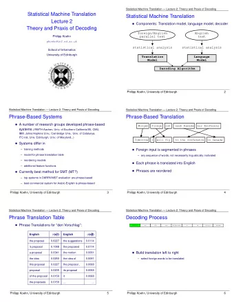
Beam Search 1. Collect all translation options: a) der Hund schläft b) der = the / that / this; Hund = dog / hound / puppy / pug ; schläft = sleeps / sleep / sleepy c) der Hund = the dog / the hound 2. Build hypotheses , starting with the empty hypothesis: 1. der = {the, that, this} 2. der Hund = {the + dog, the + hound, the + puppy, the +pug, that + dog, that + hound, that + puppy, that +pug, this + dog, this + hound, this + puppy, this +pug, the dog, the hound} 3. ... cfedermann@coli.uni-saarland.de Language Technology II (SS 2013): Machine Translation 4
Beam Search II In the end, we consider those hypotheses which cover the entire input sequence. Each hypothesis is annotated with the probability score that comes from using those translation options and the language model score. The hypothesis with the best score is our final translation. cfedermann@coli.uni-saarland.de Language Technology II (SS 2013): Machine Translation 5
Search Space Examining the entire search space is too expensive: it has exponential complexity. We need to reduce the complexity of the decoding problem. Two approaches: Hypothesis recombination Pruning cfedermann@coli.uni-saarland.de Language Technology II (SS 2013): Machine Translation 6
Hypothesis Recombination Translation options can create identical (partial) hypotheses: the + dog vs. the dog We can share common parts by pointing to the same final result: [the dog] ... But the probability scores will be different: using two options will yield a different score than using only one (larger) option. à drop the lower-scoring option à can never be part of the best-scoring hypothesis cfedermann@coli.uni-saarland.de Language Technology II (SS 2013): Machine Translation 7
Pruning If we encounter a partial hypothesis that‘s apparently worse, we want to drop it to avoid wasting computational power. But: the hypothesis might redeem itself later on and increase its probability score. We don‘t want to prune too early or too eagerly to avoid search errors. But we can only know for sure that a hypothesis is bad if we construct it completely. We need to make some educated guesses . cfedermann@coli.uni-saarland.de Language Technology II (SS 2013): Machine Translation 8
Stack Decoding Organise hypotheses in stacks. Order them e.g. by number of words translated. Only if the number grows too large, drop the worst hypotheses. But: is the sorting (number of translated words, ...) enough to tell how good a hypothesis is? cfedermann@coli.uni-saarland.de Language Technology II (SS 2013): Machine Translation 9
Pruning Methods I Histogram pruning: Keep N hypotheses in the stack We have stack size N, a number of translation options T and the length of the input sentence L: O (N*T*L) T is linear to L è O (N*L 2 ) cfedermann@coli.uni-saarland.de Language Technology II (SS 2013): Machine Translation 10
Pruning Methods II Threshold pruning: Considers difference in score between the best and the worst hypotheses in the stack. We declare a fixed threshold α by which a hypothesis is allowed to be worse than the best hypothesis. α declares the beam width in which we perform our search. cfedermann@coli.uni-saarland.de Language Technology II (SS 2013): Machine Translation 11
Future Cost To avoid pruning too eagerly, we cannot solely rely on the probability score. We approximate the future cost of creating the full hypothesis by the outside cost (rest cost) estimation: Translation model: look up the translation cost for a translation option from the phrasetable Language model: compile score without context (unigram, ...) We can now estimate the cheapest cost for translating any input span. è combine with probability score to sort hypotheses cfedermann@coli.uni-saarland.de Language Technology II (SS 2013): Machine Translation 12
Other Decoding Algorithms A* Search Similar to beam search Requires cost estimate to never over estimate the cost Greedy Hill-Climbing Decoding Generate a rough initial translation. Apply changes until translation can‘t be improved anymore. Finite State Transducers cfedermann@coli.uni-saarland.de Language Technology II (SS 2013): Machine Translation 13
Search Errors vs. Model Errors We need to distinguish error types when looking at wrong translations. Search error: the decoder fails to find the optimal translation candidate in the model Model error: the model itself contains erroneous entries cfedermann@coli.uni-saarland.de Language Technology II (SS 2013): Machine Translation 14
Advanced SMT models Word-based models (IBM1-5) don‘t capture enough information. The unit word is too small: use phrases instead. Phrase-based models are doing better è can capture collocations and multi-word expressions: kick the bucket = den Löffel abgeben the day after tomorrow = übermorgen cfedermann@coli.uni-saarland.de Language Technology II (SS 2013): Machine Translation 15
Phrase-Based SMT E* = argmax E P(E|F) = argmax E P(E) * P(F|E) In word-based models (IBM1): P(F|E) is defined as Σ p(f i |e j ) where f i and e j are the i-th French and j-th English word In the phrase-base models, we no longer have words as the basic units, but phrases which may contain up to n words (current state of the art uses 7-gram phrasetables): P(F|E) is now defined over phrases f i n and e j m where f i n contains the span of the i-th to the n-th French word and e j m the j-th to the m-th English word: P(F|E) = Π ϕ (f i n |e j m ) d(start i – end i-1 – 1) cfedermann@coli.uni-saarland.de Language Technology II (SS 2013): Machine Translation 16
Phrase Extraction Phrases are defined as continuous spans. The word alignment is key: we only extract phrases that form continuous spans on both sides Translation probability ϕ (f|e) is modeled as the relative frequency: ϕ (f|e) = count(e, f) / Σ fi count(e, f i ) cfedermann@coli.uni-saarland.de Language Technology II (SS 2013): Machine Translation 17
All Problems Solved? But phrase-based models have one big constraint: the length of the phrases: currently we work with 7-grams for phrases and 5-gram LMs in state of the art systems The larger the n-gram, the more data you need to prevent data sparseness We always need more and more data We need to make better use of the data we have cfedermann@coli.uni-saarland.de Language Technology II (SS 2013): Machine Translation 18
Factored Models In factored models we introduce additional information about the surface words: dangerous dog à dangerous|dangerous|JJ|n.sg dog| dog|NN|n.sg instead of the word use word|lemma|POS|morphology Factors allow us to generalise over the data: even if a word is unseen, if we have seen similar factors, this works in our favour: Haus|Haus|NN|n.sg è house|house|NN|n.sg Hauses|Haus|NN|g.sg? cfedermann@coli.uni-saarland.de Language Technology II (SS 2013): Machine Translation 19
More And More Possibilities Can use different translation models: lemma to lemma POS to POS We can even build more differentiated models: Translate lemma to lemma Translate morphology and POS Generate word form lemma and POS/morphology cfedermann@coli.uni-saarland.de Language Technology II (SS 2013): Machine Translation 20
Linguistic Information Complete freedom which information you use: lemma, morphology POS named entities ... But which information do we really need? In Arabic you can get results from using stems (first 4 characters) and morphology à cannot be generalised To get good factors/a good setup, you need to know your language(s) well cfedermann@coli.uni-saarland.de Language Technology II (SS 2013): Machine Translation 21
Factored Models - Problems To get the factors, you need a list of linguistic resources: lemmatiser part of speech tagger morphological analyser ... These resources may not always be available for your language pair of choice. Depending on which factors you use, your risk of data sparseness increases. Still suffers from many of the problems of phrase-based SMT cfedermann@coli.uni-saarland.de Language Technology II (SS 2013): Machine Translation 22
Recommend
More recommend
Explore More Topics
Stay informed with curated content and fresh updates.
