Machine Learning with Quantum-Inspired Tensor Networks E.M. - PowerPoint PPT Presentation

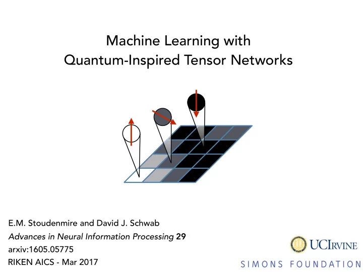
Machine Learning with Quantum-Inspired Tensor Networks E.M. Stoudenmire and David J. Schwab Advances in Neural Information Processing 29 arxiv:1605.05775 RIKEN AICS - Mar 2017

Collaboration with David J. Schwab, Northwestern and CUNY Graduate Center Quantum Machine Learning, Perimeter Institute, Aug 2016

Exciting time for machine learning Self-driving cars Language Processing Medicine Materials Science / Chemistry

Progress in neural networks and deep learning neural network diagram

Convolutional neural network "MERA" tensor network

Are tensor networks useful for machine learning? This Talk Tensor networks fit naturally into kernel learning (Also very strong connections to graphical models ) Many benefits for learning • Linear scaling • Adaptive • Feature sharing

Machine Learning Physics Topological Phases Phase Transitions Neural Nets Boltzmann Machines Quantum Monte Carlo Sign Problem Materials Science Kernel Learning & Chemistry Unsupervised Learning Tensor Networks Supervised Learning

Machine Learning Physics Topological Phases Phase Transitions Neural Nets Boltzmann Machines Quantum Monte Carlo Sign Problem Materials Science Kernel Learning & Chemistry Unsupervised Learning Tensor Networks Supervised (this talk) Learning

What are Tensor Networks?

How do tensor networks arise in physics? Quantum systems governed by Schrödinger equation: H ~ Ψ = E ~ ˆ Ψ It is just an eigenvalue problem.

The problem is that is a 2 N x 2 N matrix ˆ H ~ ⇒ wavefunction has 2 N components Ψ = ~ = E · ~ ˆ H Ψ Ψ

Natural to view wavefunction as order-N tensor Ψ s 1 s 2 s 3 ··· s N | s 1 s 2 s 3 · · · s N i X | Ψ i = { s }

Natural to view wavefunction as order-N tensor s 1 s 2 s 3 s 4 s N Ψ s 1 s 2 s 3 ··· s N =

Tensor components related to probabilities of e.g. Ising model spin configurations ↓ ↓ ↑ ↑ ↑ ↑ ↑ ↑ ↑ ↑ ↑ ↑ ↓ ↓ Ψ =

Tensor components related to probabilities of e.g. Ising model spin configurations ↓ ↓ ↓ ↓ ↓ ↑ ↑ ↓ ↑ ↑ ↓↓ ↑ ↓ Ψ =

Must find an approximation to this exponential problem s 1 s 2 s 3 s 4 s N Ψ s 1 s 2 s 3 ··· s N =

Simplest approximation (mean field / rank-1) Let spins "do their own thing" Ψ s 1 s 2 s 3 s 4 s 5 s 6 ' ψ s 1 ψ s 2 ψ s 3 ψ s 4 ψ s 5 ψ s 6 s 1 s 2 s 4 s 3 s 5 s 6 Expected values of individual spins ok No correlations

Restore correlations locally Ψ s 1 s 2 s 3 s 4 s 5 s 6 ' ψ s 1 ψ s 2 ψ s 3 ψ s 4 ψ s 5 ψ s 6 s 1 s 2 s 4 s 3 s 5 s 6

Restore correlations locally Ψ s 1 s 2 s 3 s 4 s 5 s 6 ' ψ s 1 ψ s 2 ψ s 3 ψ s 4 ψ s 5 ψ s 6 i 1 i 1 s 1 s 2 s 4 s 3 s 5 s 6

Restore correlations locally Ψ s 1 s 2 s 3 s 4 s 5 s 6 ' ψ s 1 ψ s 2 ψ s 3 ψ s 4 ψ s 5 ψ s 6 i 1 i 1 i 2 i 2 i 3 i 3 i 4 i 4 i 5 i 5 s 1 s 2 s 4 s 3 s 5 s 6 matrix product state (MPS) Local expected values accurate Correlations decay with spatial distance

↓ ↓ ↓ ↑ ↑ ↑ "Matrix product state" because retrieving an element product of matrices =

↓↓ ↓ Ψ ↑ ↑↑ = "Matrix product state" because retrieving an element product of matrices =

Tensor diagrams have rigorous meaning v j j M ij i j T ijk i k j

Joining lines implies contraction, can omit names X M ij v j i j j A ij B jk = AB = Tr[ AB ] A ij B ji

MPS = matrix product state ≈ MPS approximation controlled by bond dimension "m" (like SVD rank) Compress parameters into 2 N parameters N · 2 · m 2 can represent any tensor N m ∼ 2 2

Friendly neighborhood of "quantum state space" Ψ m=8 m=4 m=2 m=1

MPS = matrix product state MPS lead to powerful optimization techniques ( DMRG algorithm ) White, PRL 69 , 2863 (1992) Stoudenmire, White, PRB 87 , 155137 (2013)

Besides MPS, other successful tensor are PEPS and MERA MERA PEPS (2D systems) (critical systems) Evenbly, Vidal, PRB 79 , 144108 (2009) Verstraete, Cirac, cond-mat/0407066 (2004) Orus, Ann. Phys. 349 , 117 (2014)

Supervised Kernel Learning

Supervised Learning Very common task: Labeled training data (= supervised) Find decision function f ( x ) f ( x ) > 0 x ∈ A f ( x ) < 0 x ∈ B Input vector e.g. image pixels x

ML Overview Use training data to build model x 16 x 13 x 11 x 1 x 14 x 4 x 10 x 9 x 8 x 7 x 3 x 12 x 15 x 6 x 2 x 5

ML Overview Use training data to build model x 16 x 13 x 11 x 1 x 14 x 4 x 10 x 9 x 8 x 7 x 3 x 12 x 15 x 6 x 2 x 5

ML Overview Use training data to build model Generalize to unseen test data

ML Overview Popular approaches Neural Networks ⇣ �⌘ � f ( x ) = Φ 2 M 2 Φ 1 M 1 x Non-Linear Kernel Learning f ( x ) = W · Φ ( x )

Non-linear kernel learning Want to separate classes f ( x ) Linear classifier f ( x ) = W · x often insufficient ? ?

Non-linear kernel learning Apply non-linear "feature map" x → Φ ( x ) Φ

Non-linear kernel learning Apply non-linear "feature map" x → Φ ( x ) Φ Decision function f ( x ) = W · Φ ( x )

Non-linear kernel learning Φ Decision function f ( x ) = W · Φ ( x ) Linear classifier in feature space

Non-linear kernel learning Example of feature map Φ x = ( x 1 , x 2 , x 3 ) Φ ( x ) = (1 , x 1 , x 2 , x 3 , x 1 x 2 , x 1 x 3 , x 2 x 3 ) is "lifted" to feature space x

Proposal for Learning

Grayscale image data

Map pixels to "spins"

Map pixels to "spins"

Map pixels to "spins"

x = input Local feature map , dimension d=2 ⇣ π ⇣ π h ⌘ ⌘i φ ( x j ) = cos , sin x j ∈ [0 , 1] 2 x j 2 x j Crucially, grayscale values not orthogonal

x = input φ = local feature map Total feature map Φ ( x ) Φ s 1 s 2 ··· s N ( x ) = φ s 1 ( x 1 ) ⊗ φ s 2 ( x 2 ) ⊗ · · · ⊗ φ s N ( x N ) • Tensor product of local feature maps / vectors • Just like product state wavefunction of spins • Vector in dimensional space 2 N

x = input φ = local feature map Total feature map Φ ( x ) More detailed notation raw inputs x = [ x 1 , x N ] x 2 , x 3 , . . . , [ [ [ [ [ [ [ [ φ 1 ( ) φ 1 ( ) φ 1 ( ) φ 1 ( ) feature x 1 x 2 x 3 x N Φ ( x ) = ⊗ ⊗ ⊗ ⊗ . . . vector φ 2 ( ) φ 2 ( ) φ 2 ( ) φ 2 ( ) x 1 x 2 x 3 x N

x = input φ = local feature map Total feature map Φ ( x ) Tensor diagram notation raw inputs x = [ x 1 , x N ] x 2 , x 3 , . . . , s N s 2 s 3 s 4 s 5 s 6 s 1 feature vector Φ ( x ) = · · · φ s 1 φ s 2 φ s 3 φ s 4 φ s 5 φ s 6 φ s N

Construct decision function f ( x ) = W · Φ ( x ) Φ ( x )

Construct decision function f ( x ) = W · Φ ( x ) W Φ ( x )

Construct decision function f ( x ) = W · Φ ( x ) W f ( x ) = Φ ( x )

Construct decision function f ( x ) = W · Φ ( x ) W f ( x ) = Φ ( x ) W =

Main approximation order-N tensor W = matrix product ≈ state (MPS)

MPS form of decision function W f ( x ) = Φ ( x )

Linear scaling Can use algorithm similar to DMRG to optimize N = size of input Scaling is N · N T · m 3 N T = size of training set m = MPS bond dimension W f ( x ) = Φ ( x )

Linear scaling Can use algorithm similar to DMRG to optimize N = size of input Scaling is N · N T · m 3 N T = size of training set m = MPS bond dimension W f ( x ) = Φ ( x )

Linear scaling Can use algorithm similar to DMRG to optimize N = size of input Scaling is N · N T · m 3 N T = size of training set m = MPS bond dimension W f ( x ) = Φ ( x )

Linear scaling Can use algorithm similar to DMRG to optimize N = size of input Scaling is N · N T · m 3 N T = size of training set m = MPS bond dimension W f ( x ) = Φ ( x )

Linear scaling Can use algorithm similar to DMRG to optimize N = size of input Scaling is N · N T · m 3 N T = size of training set m = MPS bond dimension W f ( x ) = Φ ( x ) Could improve with stochastic gradient

Multi-class extension of model Decision function f ` ( x ) = W ` · Φ ( x ) Index runs over possible labels ` ` W ` f ` ( x ) = Φ ( x ) ` W ` = Φ ( x ) Predicted label is argmax ` | f ` ( x ) |

MNIST Experiment MNIST is a benchmark data set of grayscale handwritten digits (labels = 0,1,2,...,9) ` 60,000 labeled training images 10,000 labeled test images

MNIST Experiment One-dimensional mapping

MNIST Experiment Results Bond dimension Test Set Error ~5% (500/10,000 incorrect) m = 10 m = 20 ~2% (200/10,000 incorrect) m = 120 0.97% (97/10,000 incorrect) State of the art is < 1% test set error

MNIST Experiment Demo Link: http://itensor.org/miles/digit/index.html

Understanding Tensor Network Models W f ( x ) = Φ ( x )

Again assume is an MPS W W f ( x ) = Φ ( x ) Many interesting benefits Two are: 1. Adaptive 2. Feature sharing

1. Tensor networks are adaptive { grayscale boundary pixels not training useful for learning data