Machine Learning Review 1 Linear Regression Assume a set of traning - PDF document

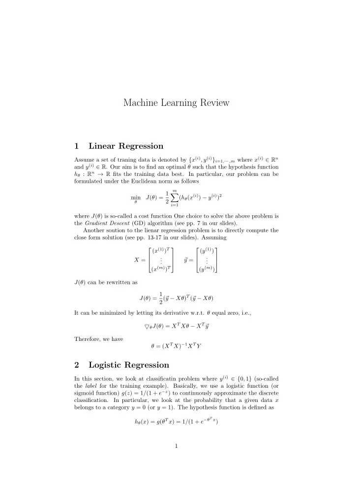
Machine Learning Review 1 Linear Regression Assume a set of traning data is denoted by { x ( i ) , y ( i ) } i =1 , ··· ,m where x ( i ) ∈ R n and y ( i ) ∈ R . Our aim is to find an optimal θ such that the hypothesis function h θ : R n → R fits the training data best. In particular, our problem can be formulated under the Euclidean norm as follows m J ( θ ) = 1 � ( h θ ( x ( i ) ) − y ( i ) ) 2 min 2 θ i =1 where J ( θ ) is so-called a cost function One choice to solve the above problem is the Gradient Descent (GD) algorithm (see pp. 7 in our slides). Another soution to the lienar regression problem is to directly compute the close form solution (see pp. 13-17 in our slides). Assuming ( x (1) ) T ( y (1) )     . . . . X = y = �     . .     ( x ( m ) ) T ( y ( m ) ) J ( θ ) can be rewritten as J ( θ ) = 1 y − Xθ ) T ( � 2( � y − Xθ ) It can be minimized by letting its derivative w.r.t. θ equal zero, i.e., ▽ θ J ( θ ) = X T Xθ − X T � y Therefore, we have θ = ( X T X ) − 1 X T Y 2 Logistic Regression In this section, we look at classificatin problem where y ( i ) ∈ { 0 , 1 } (so-called the label for the training example). Basically, we use a logistic function (or sigmoid function) g ( z ) = 1 / (1 + e − z ) to continuously approximate the discrete classification. In particular, we look at the probability that a given data x belongs to a category y = 0 (or y = 1). The hypothesis function is defined as h θ ( x ) = g ( θ T x ) = 1 / (1 + e − θ T x ) 1

Assuming p ( y = 1 | x ; θ ) = h θ ( x ) = 1 / (1 + exp( − θ T x ) p ( y = 0 | x ; θ ) = 1 − h θ ( x ) = 1 / (1 + exp( θ T x ) we have that p ( y | x ; θ ) = ( h θ ( x )) y (1 − h θ ( x )) 1 − y Given a set of training data { x ( i ) , y ( i ) } i =1 , ··· ,m , we define the likelihood func- tion as p ( y ( i ) | x ( i ) ; θ ) � L ( θ ) = i ( h θ ( x ( i ) )) y ( i ) (1 − h θ ( x ( i ) )) 1 − y ( i ) � = i To simply the computations, we take the logarithm of the likelihood function (i.e. so-called log-likelihood ) m � y ( i ) log h θ ( x ( i ) ) + (1 − y ( i ) ) log(1 − h θ ( x ( i ) ) � � ℓ ( θ ) = log L ( θ ) = i =1 We can use gradient ascent algorithm to maximize the above objective function (see pp. 10 in our slides). Also, we can take another choice, i.e., Newton’s method (see. pp. 11-13 in our slides) 3 Regularization and Bayesian Statistics We first take the linear regression problem for an example. To sovle the overfit- ting problem, we introduce a regularization item (or penalty) in the objective function, i.e.,   m n 1 ( h θ ( x ( i ) ) − y ( i ) ) 2 + λ � � θ 2 min   j 2 m θ i =1 j =1 A gradient descent based solution is given on pp. 7 in our slides. Also, the closed form solution can be found on pp. 9. As shown on pp. 10, similar method can be applied to logistic regression problem. We then look at Maximum Likelihood Estimation (MLE). Assume data are generated via probability distribution d ∼ p ( d | θ ) Given a set of independent and identically distributed (i.i.d.) data samples D = { d i } i =1 , ··· ,m , our goal is to estimate θ that best models the data. The log-likelihood function is defined by m m � � ℓ ( θ ) = log p ( d i | θ ) = p ( d i | θ ) i =1 i =1 Our problem becomes m � θ MLE = arg max ℓ ( θ ) = arg max p ( d i | θ ) θ θ i =1 2

In Maximum-a-Posteriori Estimation (MAP), we treat θ as a random vari- able. Our goal is to choose θ that maximizes the posterior probability of θ (i.e., probability in the light of the observed data). According to Bayes rule p ( θ | D ) = p ( θ ) p ( D | θ ) p ( D ) Note that, p ( D ) is independent of θ . In MAP, our problem is formulated by θ MAP = arg max p ( θ | D ) θ p ( θ ) p ( D | θ ) = arg max p ( D ) θ = arg max p ( θ ) p ( D | θ ) θ = arg max log p ( θ ) p ( D | θ ) θ = arg max (log p ( θ ) + log p ( D | θ )) θ � m � � = arg max log p ( θ ) + log p ( d i | θ ) θ i =1 The detailed application of MLE and MAP to linear regression and logistic regression can be found in pp. 15-22. 4 Naive Bayes and EM Algorithm Given a set of training data, the features and labels are both represented by random variables { X j } j =1 , ··· ,n and Y , respectively. The key of Naive Bayes is to assume that X j and X j ′ are conditionally independent given Y , for ∀ j � = j ′ . Hence, given a data sample x = [ x 1 , x 2 , · · · , x n ] and its label y , we have that P ( X 1 = x 1 , X 2 = x 2 , · · · , X n = x n | Y = y ) n � = P ( X j = x j | X 1 = x 1 , X 2 = x 2 , · · · , X j − 1 = x j − 1 , Y = y ) j =1 n � = P ( X j = x j | Y = y ) j =1 Then the Naive Bayes model can be formulated as P ( Y = y | X 1 = x 1 , · · · , X n = x n ) P ( X 1 = x 1 , · · · , X n = x n | Y = y ) p ( Y = y ) = P ( X 1 = x 1 , · · · , X n = x n ) P ( Y = y ) � n j =1 p ( X j = x j | Y = y ) = P ( X 1 = x 1 , · · · , X n = x n ) where there are two sets of parameters (denoted by Ω): p ( Y = y ) (or p ( y )) and p ( X j = x | Y = y ) (or p j ( x | y )). Since p ( X 1 = x 1 , · · · , X n = x n ) follows a predefined distribution and is independent of these parameters, we have that n � p ( y | x 1 , · · · , x n ) ∝ p ( y ) p j ( x j | y ) j =1 3

Given a set of training data { x ( i ) , y ( i ) } , the log-likelihood function is m � log p ( x ( i ) , y ( i ) ) ℓ (Ω) = i =1   m n � � p j ( x ( i )  p ( y ( i ) ) | y ( i ) ) = log  j i =1 j =1 m m n � � � log p j ( x ( i ) log p ( y ( i ) ) + | y ( i ) ) = j i =1 i =1 j =1 The maximum-likelihood estimates are then the parameter values p ( y ) and p j ( x j | y ) that maximize m m n � � � log p j ( x ( i ) log p ( y ( i ) ) + | y ( i ) ) ℓ (Ω) = j i =1 i =1 j =1 subject to the following constraints: • p ( y ) ≥ 0 for ∀ y ∈ { 1 , 2 , · · · , k } • � k y =1 p ( y ) = 1 • For ∀ y ∈ { 1 , · · · , k } , j ∈ { 1 , · · · , n } , x ∈ { 0 , 1 } , p j ( x | y ) ≥ 0 • For ∀ y ∈ { 1 , · · · , k } , j ∈ { 1 , · · · , n } , � x ∈{ 0 , 1 } p j ( x | y ) = 1 Solutions can be found on pp. 49 in our slides. In the Expectation-Maximization (EM) algorithm, we assume there is no label for any training data. By introducing a latent variable z , the log-likelihood function can be defined as m m � � � log p ( x ( i ) ; θ ) = p ( x ( i ) , z ; θ ) ℓ ( θ ) = log z i =1 i =1 The basic idea of EM algorithm (to maximizing ℓ ( θ )) is to repeatedly construct a lower-bound on ℓ (E-step), and then optimize that lower-bound (M-step) For each i ∈ { 1 , 2 , · · · , m } , let Q i be some distribution over the z ’s � Q i ( z ) = 1 , Q i ( z ) ≥ 0 z We have m � � p ( x ( i ) , z ( i ) ; θ ) ℓ ( θ ) = log i =1 z ( i ) m Q i ( z ( i ) ) p ( x ( i ) , z ( i ) ; θ ) � � = log Q i ( z ( i ) ) i =1 z ( i ) m Q i ( z ( i ) ) log p ( x ( i ) , z ( i ) ; θ ) � � ≥ Q i ( z ( i ) ) i =1 z ( i ) 4

since � p ( x ( i ) , z ( i ) ; θ ) � p ( x ( i ) , z ( i ) ; θ ) � �� � �� log E z ( i ) ∼ Q i ≥ E z ( i ) ∼ Q i log Q i ( z ( i ) ) Q i ( z ( i ) ) according to the Jensen’s inequality (see pp. 25 for the details of Jensen’s inequality). Therefore, for any set of distributions Q i , ℓ ( θ ) has a lower bound m Q i ( z ( i ) ) log p ( x ( i ) , z ( i ) ; θ ) � � Q i ( z ( i ) ) i =1 z ( i ) In order to tighten the lower bound (i.e., to let the equality hold in the Jensen’s inequality), p ( x ( i ) , z ( i ) ; θ ) /Q i ( z ( i ) ) should be a constant (such that E[ p ( x ( i ) , z ( i ) ; θ ) /Q i ( z ( i ) )] = p ( x ( i ) , z ( i ) ; θ ) /Q i ( z ( i ) )). Therefore, Q i ( z ( i ) ) ∝ p ( x, z ( i ) ; θ ) Since � z Q i ( z ) = 1, one natural choice is p ( x ( i ) , z ( i ) ; θ ) Q i ( z ( i ) ) = � z p ( x ( i ) , z ( i ) ; θ ) p ( x ( i ) , z ( i ) ; θ ) = p ( x ( i ) ; θ ) p ( z ( i ) | x ( i ) ; θ ) = In EM algorithm, we repeat the following step until convergence • (E-step) For each i , set Q i ( z ( i ) ) := p ( z ( i ) | x ( i ) ; θ ) • (M-step) set Q i ( z ( i ) ) log p ( x ( i ) , z ( i ) ; θ ) � � θ := arg max Q i ( z ( i ) ) θ i z ( i ) The convergence of the EM algorithm can be found on pp. 95 in our slides. An example of applying the EM algorithm to the Mixtures of Gaussians is given on pp. 98-105. Also, as shown on pp. 106-115, EM algorithm also can be applied to Naive Bayes model. 5 SVM In SVM, we use a hyperplane ( w T x + b = 0) to separate the given training data. We first assume the training data is linearly separable. Give a training data x ( i ) , the margin γ ( i ) is the distance between x ( i ) and the hyperplane � w � T � x ( i ) − γ ( i ) w � b + b = 0 ⇒ γ ( i ) = x ( i ) + w T � w � � w � � w � 5