Machine Learning: Joy of Data Sarath Chandar University of - PowerPoint PPT Presentation
Machine Learning: Joy of Data Sarath Chandar University of Montreal Regression Predict my houses price ! Price Prediction Size in feet 2 ( x ) Training set of Price ($) in 1000's ( y ) 2104 460 housing prices 1416 232 (Portland, OR)
Machine Learning: Joy of Data Sarath Chandar University of Montreal
Regression
Predict my house’s price !
Price Prediction Size in feet 2 ( x ) Training set of Price ($) in 1000's ( y ) 2104 460 housing prices 1416 232 (Portland, OR) 1534 315 852 178 … … Notation: m = Number of training examples x ’s = “input” variable / features y ’s = “output” variable / “target” variable
Linear Regression Training Set Learning Algorithm Size of Estimated h house price
Linear Regression Size in feet 2 ( x ) Price ($) in 1000's ( y ) Training Set 2104 460 1416 232 1534 315 852 178 … … Hypothesis: ‘s: Parameters How to choose ‘s ?
Linear Regression 3 3 3 2 2 2 1 1 1 0 0 0 0 1 2 3 0 1 2 3 0 1 2 3
Linear Regression y x Idea: Choose so that is close to for our training examples
Linear Regression Hypothesis: Parameters: Cost Function: Goal:
Linear Regression
Gradient Descent Have some function Want Outline: • Start with some • Keep changing to reduce until we hopefully end up at a minimum
Gradient Descent J( 0 , 1 ) 1 0
Gradient Descent J( 0 , 1 ) 1 0
Gradient Descent Gradient descent algorithm
Gradient Descent If α is too small, gradient descent can be slow. If α is too large, gradient descent can overshoot the minimum. It may fail to converge, or even diverge.
Gradient Descent Gradient descent can converge to a local minimum, even with the learning rate α fixed. As we approach a local minimum, gradient descent will automatically take smaller steps. So, no need to decrease α over time.
Gradient Descent Gradient descent algorithm update and simultaneously
(for fixed , this is a function of x) (function of the parameters )
(for fixed , this is a function of x) (function of the parameters )
(for fixed , this is a function of x) (function of the parameters )
(for fixed , this is a function of x) (function of the parameters )
(for fixed , this is a function of x) (function of the parameters )
(for fixed , this is a function of x) (function of the parameters )
(for fixed , this is a function of x) (function of the parameters )
(for fixed , this is a function of x) (function of the parameters )
(for fixed , this is a function of x) (function of the parameters )
Classification
Classification: Definition • Given a collection of records ( training set ) – Each record contains a set of attributes , one of the attributes is the class . • Find a model for class attribute as a function of the values of other attributes. • Goal: previously unseen records should be assigned a class as accurately as possible. – A test set is used to determine the accuracy of the model. Usually, the given data set is divided into training and test sets, with training set used to build the model and test set used to validate it.
Illustrating Classification Task Learning Tid Attrib1 Attrib2 Attrib3 Class 1 Yes Large 125K No algorithm 2 No Medium 100K No No 3 No Small 70K 4 Yes Medium 120K No Induction 5 No Large 95K Yes 6 No Medium 60K No Learn 7 Yes Large 220K No Model Yes 8 No Small 85K 9 No Medium 75K No 10 No Small 90K Yes Model 10 Training Set Apply Model Tid Attrib1 Attrib2 Attrib3 Class 11 No Small 55K ? 12 Yes Medium 80K ? Deduction ? 13 Yes Large 110K 14 No Small 95K ? 15 No Large 67K ? 10 Test Set
Examples of Classification Task • Predicting tumor cells as benign or malignant • Classifying credit card transactions as legitimate or fraudulent • Classifying secondary structures of protein as alpha-helix, beta-sheet, or random coil • Categorizing news stories as finance, weather, entertainment, sports, etc
Clustering
Cluster Analysis • Finding groups of objects such that the objects in a group will be similar (or related) to one another and different from (or unrelated to) the objects in other groups Inter-cluster Intra-cluster distances are distances are maximized minimized
Applications of Cluster Analysis Discovered Clusters Industry Group Understanding Applied-Matl-DOWN,Bay-Network-Down,3-COM-DOWN, 1 Cabletron-Sys-DOWN,CISCO-DOWN,HP-DOWN, DSC-Comm-DOWN,INTEL-DOWN,LSI-Logic-DOWN, Technology1-DOWN – Group related documents for Micron-Tech-DOWN,Texas-Inst-Down,Tellabs-Inc-Down, Natl-Semiconduct-DOWN,Oracl-DOWN,SGI-DOWN, Sun-DOWN browsing, group genes and Apple-Comp-DOWN,Autodesk-DOWN,DEC-DOWN, 2 ADV-Micro-Device-DOWN,Andrew-Corp-DOWN, Computer-Assoc-DOWN,Circuit-City-DOWN, proteins that have similar Technology2-DOWN Compaq-DOWN, EMC-Corp-DOWN, Gen-Inst-DOWN, Motorola-DOWN,Microsoft-DOWN,Scientific-Atl-DOWN functionality, or group stocks Fannie-Mae-DOWN,Fed-Home-Loan-DOWN, 3 MBNA-Corp-DOWN,Morgan-Stanley-DOWN Financial-DOWN with similar price fluctuations Baker-Hughes-UP,Dresser-Inds-UP,Halliburton-HLD-UP, 4 Louisiana-Land-UP,Phillips-Petro-UP,Unocal-UP, Oil-UP Schlumberger-UP Summarization – Reduce the size of large data sets
Notion of a Cluster can be Ambiguous How many clusters? Six Clusters Two Clusters Four Clusters
Types of Clustering • A clustering is a set of clusters • Important distinction between hierarchical and partitional sets of clusters • Partitional Clustering – A division data objects into non-overlapping subsets (clusters) such that each data object is in exactly one subset • Hierarchical clustering – A set of nested clusters organized as a hierarchical tree
Partitional Clustering Original Points A Partitional Clustering
Hierarchical Clustering p1 p3 p4 p2 p1 p2 p3 p4 Traditional Hierarchical Clustering Traditional Dendrogram p1 p3 p4 p2 p1 p2 p3 p4 Non-traditional Hierarchical Non-traditional Dendrogram Clustering
Types of clusters : Well Seperated • Well-Separated Clusters: – A cluster is a set of points such that any point in a cluster is closer (or more similar) to every other point in the cluster than to any point not in the cluster. 3 well-separated clusters
Types of Clusters : Center-Based • Center-based – A cluster is a set of objects such that an object in a cluster is closer (more similar) to the “center” of a cluster, than to the center of any other cluster – The center of a cluster is often a centroid, the average of all the points in the cluster, or a medoid , the most “representative” point of a cluster 4 center-based clusters
Types of Clusters : Contiguity Based • Contiguous Cluster (Nearest neighbor or Transitive) – A cluster is a set of points such that a point in a cluster is closer (or more similar) to one or more other points in the cluster than to any point not in the cluster. 8 contiguous clusters
Types of Clusters : Density-Based • Density-based – A cluster is a dense region of points, which is separated by low- density regions, from other regions of high density. – Used when the clusters are irregular or intertwined, and when noise and outliers are present. 6 density-based clusters
Types of Clusters : Conceptual clusters • Shared Property or Conceptual Clusters – Finds clusters that share some common property or represent a particular concept. . 2 Overlapping Circles
Clustering Algorithms • K-means and its variants • Density-based clustering • Hierarchical clustering
K-means clustering • Partitional clustering approach. • Each cluster is associated with a centroid (center point) • Each point is assigned to the cluster with the closest centroid • Number of clusters, K, must be specified • The basic algorithm is very simple
K-means clustering : Details • Initial centroids are often chosen randomly. – Clusters produced vary from one run to another. • The centroid is (typically) the mean of the points in the cluster. • ‘Closeness’ is measured by Euclidean distance, cosine similarity, correlation, etc. • K-means will converge for common similarity measures mentioned above. • Most of the convergence happens in the first few iterations. – Often the stopping condition is changed to ‘Until relatively few points change clusters ’
Two different K-means Clusterings 3 2.5 Original Points 2 1.5 y 1 0.5 0 -2 -1.5 -1 -0.5 0 0.5 1 1.5 2 x 3 3 2.5 2.5 2 2 1.5 1.5 y y 1 1 0.5 0.5 0 0 -2 -1.5 -1 -0.5 0 0.5 1 1.5 2 -2 -1.5 -1 -0.5 0 0.5 1 1.5 2 x x Optimal Clustering Sub-optimal Clustering
An Example
Iteration 1 3 2.5 2 1.5 y 1 0.5 0 -2 -1.5 -1 -0.5 0 0.5 1 1.5 2 x
Iteration 2 3 2.5 2 1.5 y 1 0.5 0 -2 -1.5 -1 -0.5 0 0.5 1 1.5 2 x
Iteration 3 3 2.5 2 1.5 y 1 0.5 0 -2 -1.5 -1 -0.5 0 0.5 1 1.5 2 x
Iteration 4 3 2.5 2 1.5 y 1 0.5 0 -2 -1.5 -1 -0.5 0 0.5 1 1.5 2 x
Iteration 5 3 2.5 2 1.5 y 1 0.5 0 -2 -1.5 -1 -0.5 0 0.5 1 1.5 2 x
Recommend
More recommend
Explore More Topics
Stay informed with curated content and fresh updates.
