Machine learning for CalabiYau manifolds Harold Erbin Asc , Lmu - PowerPoint PPT Presentation
Machine learning for CalabiYau manifolds Harold Erbin Asc , Lmu (Germany) Machine Learning Landscape, Ictp , Trieste 12th December 2018 1 / 35 Outline: 1. Motivations Motivations Machine learning CalabiYau 3-folds Data analysis ML
Machine learning for Calabi–Yau manifolds Harold Erbin Asc , Lmu (Germany) Machine Learning Landscape, Ictp , Trieste – 12th December 2018 1 / 35
Outline: 1. Motivations Motivations Machine learning Calabi–Yau 3-folds Data analysis ML analysis Conclusion 2 / 35
String phenomenology Goal Find “the” Standard Model from string theory. Method: ◮ type II / heterotic strings, M-theory, F-theory: D = 10 , 11 , 12 ◮ vacuum choice (flux compactification): ◮ (typically) Calabi–Yau (CY) 3- or 4-fold ◮ fluxes and intersecting branes → reduction to D = 4 ◮ check consistency (tadpole, susy. . . ) ◮ read the D = 4 QFT (gauge group, spectrum. . . ) 3 / 35
String phenomenology Goal Find “the” Standard Model from string theory. Method: ◮ type II / heterotic strings, M-theory, F-theory: D = 10 , 11 , 12 ◮ vacuum choice (flux compactification): ◮ (typically) Calabi–Yau (CY) 3- or 4-fold ◮ fluxes and intersecting branes → reduction to D = 4 ◮ check consistency (tadpole, susy. . . ) ◮ read the D = 4 QFT (gauge group, spectrum. . . ) No vacuum selection mechanism ⇒ string landscape 3 / 35
Landscape mapping String phenomenology: ◮ find consistent string models ◮ find generic/common features ◮ reproduce the Standard Model 4 / 35
Landscape mapping String phenomenology: ◮ find consistent string models ◮ find generic/common features ◮ reproduce the Standard Model Typical challenges: properties and equations involving many integers 4 / 35
Types of data Calabi–Yau (CY) manifolds ◮ CICY (complete intersection in products of projective spaces): 7890 (3-fold), 921 , 497 (4-fold) ◮ Kreuzer–Skarke (reflexive polyhedra): 473 , 800 , 776 ( d = 4) String and F-theory models involve huge numbers ◮ 10 500 ◮ 10 755 ◮ 10 272 , 000 ◮ . . . 5 / 35
Types of data Calabi–Yau (CY) manifolds ◮ CICY (complete intersection in products of projective spaces): 7890 (3-fold), 921 , 497 (4-fold) ◮ Kreuzer–Skarke (reflexive polyhedra): 473 , 800 , 776 ( d = 4) String and F-theory models involve huge numbers ◮ 10 500 ◮ 10 755 ◮ 10 272 , 000 ◮ . . . → use machine learning 5 / 35
Plan Analysis of CICY 3-fold ◮ ML methodology ◮ results and discussions of Hodge numbers In progress with: Vincent Lahoche, Mohamed El Amine Seddik, Mohamed Tamaazousti ( List , Cea ). 6 / 35
Outline: 2. Machine learning Motivations Machine learning Calabi–Yau 3-folds Data analysis ML analysis Conclusion 7 / 35
Definition Machine learning (Samuel) The field of study that gives computers the ability to learn without being explicitly programmed. Machine learning (Mitchell) A computer program is said to learn from experience E with respect to some class of tasks T and performance measure P if its performance at tasks in T , as measured by P , improves with experience E . 8 / 35
Deep neural network Architecture: ◮ 1–many hidden layers ◮ link: weighted input ◮ neuron: non-linear "activation function" Summary: x ( n +1) = g ( n +1) ( W ( n ) x ( n ) ). Generic method: fixed functions g ( n ) , learn weights W ( n ) 9 / 35
Deep neural network x (1) ≡ x i 1 i 1 x (2) = g (2) � W (1) i 2 i 1 x (1) � i 2 i 1 f i 3 ( x i 1 ) ≡ x (3) = g (3) � W (2) i 3 i 2 x (2) � i 3 i 2 i 1 = 1 , 2 , 3; i 2 = 1 , . . . , 4; i 3 = 1 , 2 Summary: x ( n +1) = g ( n +1) ( W ( n ) x ( n ) ). Generic method: fixed functions g ( n ) , learn weights W ( n ) 9 / 35
Learning method ◮ define a loss function L N train � y (train) , y (pred) � � L = distance i i i =1 ◮ minimize the loss function (iterated gradient descent. . . ) 10 / 35
Learning method ◮ define a loss function L N train � y (train) , y (pred) � � L = distance i i i =1 ◮ minimize the loss function (iterated gradient descent. . . ) ◮ main risk: overfitting (= cannot generalize) → various solutions (regularization, dropout. . . ) → split data set in two (training and test) 10 / 35
ML workflow “Naive” workflow: 1. get raw data 2. write neural network with many layers 3. feed raw data to neural network 4. get nice results (or give up) 11 / 35
ML workflow Real-world workflow: 1. understand the problem 2. exploratory data analysis ◮ feature engineering ◮ feature selection 3. baseline model ◮ full working pipeline ◮ lower-bound on accuracy 4. validation strategy 5. machine learning model 6. ensembling Pragmatic ref.: coursera.org/learn/competitive-data-science 11 / 35
Complex neural network 12 / 35
Complex neural network Particularities: ◮ f i ( I ) : engineered features ◮ identical outputs (stabilisation) 12 / 35
Outline: 3. Calabi–Yau 3-folds Motivations Machine learning Calabi–Yau 3-folds Data analysis ML analysis Conclusion 13 / 35
Calabi-Yau Complete intersection Calabi–Yau (CICY) 3-fold: ◮ CY: complex manifold with vanishing first Chern class ◮ complete intersection: non-degenerate hypersurface in products of projective spaces ◮ hypersurface = solution to system of homogeneous polynomial equations 14 / 35
Calabi-Yau Complete intersection Calabi–Yau (CICY) 3-fold: ◮ CY: complex manifold with vanishing first Chern class ◮ complete intersection: non-degenerate hypersurface in products of projective spaces ◮ hypersurface = solution to system of homogeneous polynomial equations ◮ described by configuration matrix m × k a 1 a 1 P n 1 · · · 1 k . . . ... . . . X = . . . P n m a m a m · · · 1 k m k � � a r dim C X = n r − k = 3 , n r + 1 = α r =1 α =1 α power of coordinates on P n r in α th equation ◮ a r 14 / 35
Configuration matrix Examples ◮ quintic ( X a ) 5 = 0 � � P 4 � 5 = ⇒ x a ◮ 2 projective spaces, 3 equations f abc X a X b X c = 0 � � P 3 3 0 1 g αβγ Y α Y β Y γ = 0 x = ⇒ P 3 0 3 1 y h a α X a Y α = 0 15 / 35
Configuration matrix Examples ◮ quintic ( X a ) 5 = 0 � � P 4 � 5 = ⇒ x a ◮ 2 projective spaces, 3 equations f abc X a X b X c = 0 � � P 3 3 0 1 g αβγ Y α Y β Y γ = 0 x = ⇒ P 3 0 3 1 y h a α X a Y α = 0 Classification ◮ invariances (→ huge redundancy) ◮ permutation of lines and columns ◮ identities between subspaces ◮ but: ◮ constraints ⇒ bound on matrix size ◮ ∃ “favourable” configuration 15 / 35
Topology Why topology? ◮ no metric known for compact CY (cannot perform KK reduction explicitly) ◮ topological numbers → 4d properties (number of fields, representations, gauge symmetry. . . ) 16 / 35
Topology Why topology? ◮ no metric known for compact CY (cannot perform KK reduction explicitly) ◮ topological numbers → 4d properties (number of fields, representations, gauge symmetry. . . ) Topological properties ◮ Hodge numbers h p , q (number of harmonic ( p , q )-forms) here: h 1 , 1 , h 2 , 1 ◮ Euler number χ = 2( h 11 − h 21 ) ◮ Chern classes ◮ triple intersection numbers ◮ line bundle cohomologies 16 / 35
Topology Why topology? ◮ no metric known for compact CY (cannot perform KK reduction explicitly) ◮ topological numbers → 4d properties (number of fields, representations, gauge symmetry. . . ) Topological properties ◮ Hodge numbers h p , q (number of harmonic ( p , q )-forms) here: h 1 , 1 , h 2 , 1 ◮ Euler number χ = 2( h 11 − h 21 ) ◮ Chern classes ◮ triple intersection numbers ◮ line bundle cohomologies 16 / 35
Datasets CICY have been classified ◮ 7890 configurations (but ∃ redundancies) ◮ number of product spaces: 22 ◮ h 1 , 1 ∈ [0 , 19], h 2 , 1 ∈ [0 , 101] ◮ 266 combinations ( h 1 , 1 , h 2 , 1 ) ◮ a r α ∈ [0 , 5] Original [Candelas-Dale-Lutken-Schimmrigk ’88][Green-Hubsch-Lutken ’89] ◮ maximal size: 12 × 15 ◮ number of favourable matrices: 4874 Favourable [1708.07907, Anderson-Gao-Gray-Lee] ◮ maximal size: 15 × 18 ◮ number of favourable matrices: 7820 17 / 35
Data h11 10 3 10 2 350 100 frequency 300 10 1 80 250 10 0 60 200 h21 150 10 1 40 0.0 2.5 5.0 7.5 10.0 12.5 15.0 17.5 h 11 100 20 h21 50 0 10 2 0 5 10 15 h11 frequency 10 1 Sizes Sizes 1 1 10 10 100 100 500 500 10 0 10 1 0 20 40 60 80 100 h 21 18 / 35
Goal and methodology Philosophy Start with the original dataset, derive everything else from configuration matrix and machine learning only. Current goal Input: configuration matrix − → Output: Hodge numbers 1. CICY: well studied, all topological quantities known → use as a sandbox 2. h 2 , 1 : more difficult than h 1 , 1 → prepare for studying CICY 4-folds 3. both original and favourable datasets Continue the analysis from: [1706.02714, He] [1806.03121, Bull-He-Jejjala-Mishra] 19 / 35
Outline: 4. Data analysis Motivations Machine learning Calabi–Yau 3-folds Data analysis ML analysis Conclusion 20 / 35
Feature engineering Process of creating new features derived from the raw input data. Some examples: ◮ number of projective spaces (rows), m = num _ cp ◮ number of equations (columns), k ◮ number of C P 1 ◮ number of C P 2 ◮ number of C P n with n � = 1 ◮ Frobenius norm of the matrix ◮ list of the projective space dimensions and statistics thereof (min, max, mean, median) ◮ K -nearest neighbour (KNN) clustering (with K = 2 , . . . , 5) 21 / 35
Recommend
More recommend
Explore More Topics
Stay informed with curated content and fresh updates.
