Machine-Assisted Proofs James Davenport (moderator) Bjorn Poonen - PowerPoint PPT Presentation
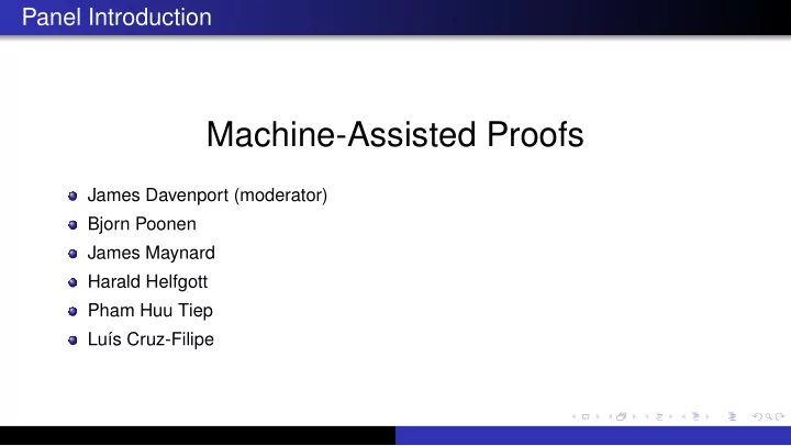
Panel Introduction Machine-Assisted Proofs James Davenport (moderator) Bjorn Poonen James Maynard Harald Helfgott Pham Huu Tiep Lu s Cruz-Filipe A (very brief, partial) history 1963 Solvability of Groups of Odd Order: 254 pages
Rigorous computations Rigorous computations with real numbers must take into account rounding errors. Moreover, a generic element of R cannot even be represented in bounded space. Interval arithmetic provides a way to keep track of rounding errors automatically, while providing data types for work in R and C . The basic data type is an interval [ a , b ] , where a , b ∈ Q . Of course, rationals can be stored in a computer. Best if of the form n / 2 k .
Rigorous computations Rigorous computations with real numbers must take into account rounding errors. Moreover, a generic element of R cannot even be represented in bounded space. Interval arithmetic provides a way to keep track of rounding errors automatically, while providing data types for work in R and C . The basic data type is an interval [ a , b ] , where a , b ∈ Q . Of course, rationals can be stored in a computer. Best if of the form n / 2 k . A procedure is said to implement a function f : R k → R if, given B = ([ a i , b i ]) 1 ≤ i ≤ k ⊂ R k , it returns an interval in R containing f ( B ) .
Rigorous computations Rigorous computations with real numbers must take into account rounding errors. Moreover, a generic element of R cannot even be represented in bounded space. Interval arithmetic provides a way to keep track of rounding errors automatically, while providing data types for work in R and C . The basic data type is an interval [ a , b ] , where a , b ∈ Q . Of course, rationals can be stored in a computer. Best if of the form n / 2 k . A procedure is said to implement a function f : R k → R if, given B = ([ a i , b i ]) 1 ≤ i ≤ k ⊂ R k , it returns an interval in R containing f ( B ) . First proposed in the late 1950s. Several commonly used open-source implementations.
Rigorous computations Rigorous computations with real numbers must take into account rounding errors. Moreover, a generic element of R cannot even be represented in bounded space. Interval arithmetic provides a way to keep track of rounding errors automatically, while providing data types for work in R and C . The basic data type is an interval [ a , b ] , where a , b ∈ Q . Of course, rationals can be stored in a computer. Best if of the form n / 2 k . A procedure is said to implement a function f : R k → R if, given B = ([ a i , b i ]) 1 ≤ i ≤ k ⊂ R k , it returns an interval in R containing f ( B ) . First proposed in the late 1950s. Several commonly used open-source implementations. (The package ARB implements a variant, ball arithmetic .)
Rigorous computations Rigorous computations with real numbers must take into account rounding errors. Moreover, a generic element of R cannot even be represented in bounded space. Interval arithmetic provides a way to keep track of rounding errors automatically, while providing data types for work in R and C . The basic data type is an interval [ a , b ] , where a , b ∈ Q . Of course, rationals can be stored in a computer. Best if of the form n / 2 k . A procedure is said to implement a function f : R k → R if, given B = ([ a i , b i ]) 1 ≤ i ≤ k ⊂ R k , it returns an interval in R containing f ( B ) . First proposed in the late 1950s. Several commonly used open-source implementations. (The package ARB implements a variant, ball arithmetic .) Cost: multiplies running time by (very roughly) ∼ 10 (depending on the implementation).
Rigorous computations Rigorous computations with real numbers must take into account rounding errors. Moreover, a generic element of R cannot even be represented in bounded space. Interval arithmetic provides a way to keep track of rounding errors automatically, while providing data types for work in R and C . The basic data type is an interval [ a , b ] , where a , b ∈ Q . Of course, rationals can be stored in a computer. Best if of the form n / 2 k . A procedure is said to implement a function f : R k → R if, given B = ([ a i , b i ]) 1 ≤ i ≤ k ⊂ R k , it returns an interval in R containing f ( B ) . First proposed in the late 1950s. Several commonly used open-source implementations. (The package ARB implements a variant, ball arithmetic .) Cost: multiplies running time by (very roughly) ∼ 10 (depending on the implementation). Example of a large-scale application: D. Platt’s verification of the Riemann Hypothesis for zeroes with imaginary part ≤ 1 . 1 · 10 11 .
Rigorous computations Rigorous computations with real numbers must take into account rounding errors. Moreover, a generic element of R cannot even be represented in bounded space. Interval arithmetic provides a way to keep track of rounding errors automatically, while providing data types for work in R and C . The basic data type is an interval [ a , b ] , where a , b ∈ Q . Of course, rationals can be stored in a computer. Best if of the form n / 2 k . A procedure is said to implement a function f : R k → R if, given B = ([ a i , b i ]) 1 ≤ i ≤ k ⊂ R k , it returns an interval in R containing f ( B ) . First proposed in the late 1950s. Several commonly used open-source implementations. (The package ARB implements a variant, ball arithmetic .) Cost: multiplies running time by (very roughly) ∼ 10 (depending on the implementation). Example of a large-scale application: D. Platt’s verification of the Riemann Hypothesis for zeroes with imaginary part ≤ 1 . 1 · 10 11 . Note: It is possible to avoid interval arithmetic and keep track of rounding erros by hand.
Rigorous computations Rigorous computations with real numbers must take into account rounding errors. Moreover, a generic element of R cannot even be represented in bounded space. Interval arithmetic provides a way to keep track of rounding errors automatically, while providing data types for work in R and C . The basic data type is an interval [ a , b ] , where a , b ∈ Q . Of course, rationals can be stored in a computer. Best if of the form n / 2 k . A procedure is said to implement a function f : R k → R if, given B = ([ a i , b i ]) 1 ≤ i ≤ k ⊂ R k , it returns an interval in R containing f ( B ) . First proposed in the late 1950s. Several commonly used open-source implementations. (The package ARB implements a variant, ball arithmetic .) Cost: multiplies running time by (very roughly) ∼ 10 (depending on the implementation). Example of a large-scale application: D. Platt’s verification of the Riemann Hypothesis for zeroes with imaginary part ≤ 1 . 1 · 10 11 . Note: It is possible to avoid interval arithmetic and keep track of rounding erros by hand. Doing so would save computer time at the expense of human time, and would create one more
Rigorous computations, II: comparisons. Maxima and minima Otherwise put: making “proof by graph” rigorous.
Rigorous computations, II: comparisons. Maxima and minima Otherwise put: making “proof by graph” rigorous. Comparing functions in exploratory work:
Rigorous computations, II: comparisons. Maxima and minima Otherwise put: making “proof by graph” rigorous. Comparing functions in exploratory work: f ( x ) ≤ g ( x ) for x ∈ [ 0 , 1 ] because a plot tells me so.
Rigorous computations, II: comparisons. Maxima and minima Otherwise put: making “proof by graph” rigorous. Comparing functions in exploratory work: f ( x ) ≤ g ( x ) for x ∈ [ 0 , 1 ] because a plot tells me so. Comparing functions in a proof:
Rigorous computations, II: comparisons. Maxima and minima Otherwise put: making “proof by graph” rigorous. Comparing functions in exploratory work: f ( x ) ≤ g ( x ) for x ∈ [ 0 , 1 ] because a plot tells me so. Comparing functions in a proof: must prove that f ( x ) − g ( x ) ≤ 0 for x ∈ [ 0 , 1 ] .
Rigorous computations, II: comparisons. Maxima and minima Otherwise put: making “proof by graph” rigorous. Comparing functions in exploratory work: f ( x ) ≤ g ( x ) for x ∈ [ 0 , 1 ] because a plot tells me so. Comparing functions in a proof: must prove that f ( x ) − g ( x ) ≤ 0 for x ∈ [ 0 , 1 ] . Can let the computer prove this fact! Bisection method and interval arithmetic. Look at derivatives if necessary. Similarly for: locating maxima and minima. Interval arithmetic particularly suitable.
Rigorous computations, III: numerical integration � 1 F ( x ) dx = ? 0
Rigorous computations, III: numerical integration � 1 F ( x ) dx = ? 0 It is not enough to increase the “precision” in Sagemath/Mathematica/Maple until the result seems to converge.
Rigorous computations, III: numerical integration � 1 F ( x ) dx = ? 0 It is not enough to increase the “precision” in Sagemath/Mathematica/Maple until the result seems to converge. Rigorous quadrature: use trapezoid rule, or Simpson’s rule, or Euler-Maclaurin, etc., together with interval arithmetic, using bounds on derivatives of F to bound the error.
Rigorous computations, III: numerical integration � 1 F ( x ) dx = ? 0 It is not enough to increase the “precision” in Sagemath/Mathematica/Maple until the result seems to converge. Rigorous quadrature: use trapezoid rule, or Simpson’s rule, or Euler-Maclaurin, etc., together with interval arithmetic, using bounds on derivatives of F to bound the error. What if F is pointwise not differentiable?
Rigorous computations, III: numerical integration � 1 F ( x ) dx = ? 0 It is not enough to increase the “precision” in Sagemath/Mathematica/Maple until the result seems to converge. Rigorous quadrature: use trapezoid rule, or Simpson’s rule, or Euler-Maclaurin, etc., together with interval arithmetic, using bounds on derivatives of F to bound the error. What if F is pointwise not differentiable? Should be automatic; as of the dark days of 2018, some ad-hoc work still needed.
Rigorous computations, III: numerical integration � 1 F ( x ) dx = ? 0 It is not enough to increase the “precision” in Sagemath/Mathematica/Maple until the result seems to converge. Rigorous quadrature: use trapezoid rule, or Simpson’s rule, or Euler-Maclaurin, etc., together with interval arithmetic, using bounds on derivatives of F to bound the error. What if F is pointwise not differentiable? Should be automatic; as of the dark days of 2018, some ad-hoc work still needed. Even more ad-hoc work needed for complex integrals.
Rigorous computations, III: numerical integration � 1 F ( x ) dx = ? 0 It is not enough to increase the “precision” in Sagemath/Mathematica/Maple until the result seems to converge. Rigorous quadrature: use trapezoid rule, or Simpson’s rule, or Euler-Maclaurin, etc., together with interval arithmetic, using bounds on derivatives of F to bound the error. What if F is pointwise not differentiable? Should be automatic; as of the dark days of 2018, some ad-hoc work still needed. Even more ad-hoc work needed for complex integrals. p ≤ r ( 1 − p − s ) and R the straight path from 200 i to 40000 i , Example: for P r ( s ) = � � | P ( s + 1 / 2 ) P ( s + 1 / 4 ) || ζ ( s + 1 / 2 ) || ζ ( s + 1 / 4 ) | 1 | ds | = 0 . 009269 + error , | s | 2 π i R where | error | ≤ 3 · 10 − 6 .
Rigorous computations, III: numerical integration � 1 F ( x ) dx = ? 0 It is not enough to increase the “precision” in Sagemath/Mathematica/Maple until the result seems to converge. Rigorous quadrature: use trapezoid rule, or Simpson’s rule, or Euler-Maclaurin, etc., together with interval arithmetic, using bounds on derivatives of F to bound the error. What if F is pointwise not differentiable? Should be automatic; as of the dark days of 2018, some ad-hoc work still needed. Even more ad-hoc work needed for complex integrals. p ≤ r ( 1 − p − s ) and R the straight path from 200 i to 40000 i , Example: for P r ( s ) = � � | P ( s + 1 / 2 ) P ( s + 1 / 4 ) || ζ ( s + 1 / 2 ) || ζ ( s + 1 / 4 ) | 1 | ds | = 0 . 009269 + error , | s | 2 π i R where | error | ≤ 3 · 10 − 6 . Method: e-mail ARB’s author (F. Johansson). To change the path or integrand, edit the code he sends you. Run overnight.
Algorithmic complexity. Computations and asymptotic analysis Whether an algorithm runs in time O ( N ) , O ( N 2 ) or O ( N 3 ) is much more important (for large N ) than its implementation.
Algorithmic complexity. Computations and asymptotic analysis Whether an algorithm runs in time O ( N ) , O ( N 2 ) or O ( N 3 ) is much more important (for large N ) than its implementation. Why large N ?
Algorithmic complexity. Computations and asymptotic analysis Whether an algorithm runs in time O ( N ) , O ( N 2 ) or O ( N 3 ) is much more important (for large N ) than its implementation. Why large N ? Often, methods from analysis show: expression ( n ) = f ( n ) + error , where | error | ≤ g ( n ) and g ( n ) ≪ | f ( n ) | , but only for n large.
Algorithmic complexity. Computations and asymptotic analysis Whether an algorithm runs in time O ( N ) , O ( N 2 ) or O ( N 3 ) is much more important (for large N ) than its implementation. Why large N ? Often, methods from analysis show: expression ( n ) = f ( n ) + error , where | error | ≤ g ( n ) and g ( n ) ≪ | f ( n ) | , but only for n large. For n ≤ N , we compute expression ( n ) instead. That can establish a strong, simple bound valid for all n ≤ N .
Algorithmic complexity. Computations and asymptotic analysis Whether an algorithm runs in time O ( N ) , O ( N 2 ) or O ( N 3 ) is much more important (for large N ) than its implementation. Why large N ? Often, methods from analysis show: expression ( n ) = f ( n ) + error , where | error | ≤ g ( n ) and g ( n ) ≪ | f ( n ) | , but only for n large. For n ≤ N , we compute expression ( n ) instead. That can establish a strong, simple bound valid for all n ≤ N . Example: let m ( n ) = � k ≤ n µ ( k ) / k . Then | m ( n ) | ≤ 0 . 0144 log n for n ≥ 96955 (Ramar´ e).
Algorithmic complexity. Computations and asymptotic analysis Whether an algorithm runs in time O ( N ) , O ( N 2 ) or O ( N 3 ) is much more important (for large N ) than its implementation. Why large N ? Often, methods from analysis show: expression ( n ) = f ( n ) + error , where | error | ≤ g ( n ) and g ( n ) ≪ | f ( n ) | , but only for n large. For n ≤ N , we compute expression ( n ) instead. That can establish a strong, simple bound valid for all n ≤ N . Example: let m ( n ) = � k ≤ n µ ( k ) / k . Then | m ( n ) | ≤ 0 . 0144 log n for n ≥ 96955 (Ramar´ e). A C program using interval arithmetic gives � | m ( n ) | ≤ 2 / n for all 0 < n ≤ 10 14 .
Algorithmic complexity. Computations and asymptotic analysis Whether an algorithm runs in time O ( N ) , O ( N 2 ) or O ( N 3 ) is much more important (for large N ) than its implementation. Why large N ? Often, methods from analysis show: expression ( n ) = f ( n ) + error , where | error | ≤ g ( n ) and g ( n ) ≪ | f ( n ) | , but only for n large. For n ≤ N , we compute expression ( n ) instead. That can establish a strong, simple bound valid for all n ≤ N . Example: let m ( n ) = � k ≤ n µ ( k ) / k . Then | m ( n ) | ≤ 0 . 0144 log n for n ≥ 96955 (Ramar´ e). A C program using interval arithmetic gives � | m ( n ) | ≤ 2 / n for all 0 < n ≤ 10 14 . An algorithm running in time almost linear on N for all n ≤ N is obvious here; it is not so in general.
Algorithmic complexity. Computations and asymptotic analysis Whether an algorithm runs in time O ( N ) , O ( N 2 ) or O ( N 3 ) is much more important (for large N ) than its implementation. Why large N ? Often, methods from analysis show: expression ( n ) = f ( n ) + error , where | error | ≤ g ( n ) and g ( n ) ≪ | f ( n ) | , but only for n large. For n ≤ N , we compute expression ( n ) instead. That can establish a strong, simple bound valid for all n ≤ N . Example: let m ( n ) = � k ≤ n µ ( k ) / k . Then | m ( n ) | ≤ 0 . 0144 log n for n ≥ 96955 (Ramar´ e). A C program using interval arithmetic gives � | m ( n ) | ≤ 2 / n for all 0 < n ≤ 10 14 . An algorithm running in time almost linear on N for all n ≤ N is obvious here; it is not so in general. The limitation can be running time or accuracy.
Errors In practice, computer errors are barely an issue, except perhaps for very large computations.
Errors In practice, computer errors are barely an issue, except perhaps for very large computations. Obvious approach: just run (or let others run) the same computation again, and again, possibly on different software/hardware. Doable unless many months of CPU time are needed. That is precisely the case when the probability of computer error may not be microscopic :( .
Errors In practice, computer errors are barely an issue, except perhaps for very large computations. Obvious approach: just run (or let others run) the same computation again, and again, possibly on different software/hardware. Doable unless many months of CPU time are needed. That is precisely the case when the probability of computer error may not be microscopic :( .
Errors In practice, computer errors are barely an issue, except perhaps for very large computations. Obvious approach: just run (or let others run) the same computation again, and again, possibly on different software/hardware. Doable unless many months of CPU time are needed. That is precisely the case when the probability of computer error may not be microscopic :( . Almost all of the time, the actual issue is human error: errors in programming, errors in input/output.
Errors In practice, computer errors are barely an issue, except perhaps for very large computations. Obvious approach: just run (or let others run) the same computation again, and again, possibly on different software/hardware. Doable unless many months of CPU time are needed. That is precisely the case when the probability of computer error may not be microscopic :( . Almost all of the time, the actual issue is human error: errors in programming, errors in input/output. Humans also make mistakes when they don’t use computers! conceptual mistakes, silly errors, especially in computations or tedious casework. How to avoid them?
Avoding errors: my current practice Program a great deal at first, but try to minimize the number of programs in submitted version, and keep them short.
Avoding errors: my current practice Program a great deal at first, but try to minimize the number of programs in submitted version, and keep them short. Time- and space-intensive computations: a few programs in C , available on request.
Avoding errors: my current practice Program a great deal at first, but try to minimize the number of programs in submitted version, and keep them short. Time- and space-intensive computations: a few programs in C , available on request. Small computations: Sagemath/Python code, largely included in the TeX source of the book. Short and readable.
Avoding errors: my current practice Program a great deal at first, but try to minimize the number of programs in submitted version, and keep them short. Time- and space-intensive computations: a few programs in C , available on request. Small computations: Sagemath/Python code, largely included in the TeX source of the book. Short and readable. Thanks to SageTeX: (a) input-output automated,
Avoding errors: my current practice Program a great deal at first, but try to minimize the number of programs in submitted version, and keep them short. Time- and space-intensive computations: a few programs in C , available on request. Small computations: Sagemath/Python code, largely included in the TeX source of the book. Short and readable. Thanks to SageTeX: (a) input-output automated, (b) code can be displayed in text by switching a TeX flag.
Avoding errors: my current practice Program a great deal at first, but try to minimize the number of programs in submitted version, and keep them short. Time- and space-intensive computations: a few programs in C , available on request. Small computations: Sagemath/Python code, largely included in the TeX source of the book. Short and readable. Thanks to SageTeX: (a) input-output automated, (b) code can be displayed in text by switching a TeX flag. Runs afresh whenever TeX file is compiled. Thus human errors in copying input/output and updating versions are minimized.
Avoding errors: my current practice Program a great deal at first, but try to minimize the number of programs in submitted version, and keep them short. Time- and space-intensive computations: a few programs in C , available on request. Small computations: Sagemath/Python code, largely included in the TeX source of the book. Short and readable. Thanks to SageTeX: (a) input-output automated, (b) code can be displayed in text by switching a TeX flag. Runs afresh whenever TeX file is compiled. Thus human errors in copying input/output and updating versions are minimized. Example: Hence, $f(x)\leq \sage{result1 + result2}$. Is it right to use a computer-algebra system in a proof?
Avoding errors: my current practice Program a great deal at first, but try to minimize the number of programs in submitted version, and keep them short. Time- and space-intensive computations: a few programs in C , available on request. Small computations: Sagemath/Python code, largely included in the TeX source of the book. Short and readable. Thanks to SageTeX: (a) input-output automated, (b) code can be displayed in text by switching a TeX flag. Runs afresh whenever TeX file is compiled. Thus human errors in copying input/output and updating versions are minimized. Example: Hence, $f(x)\leq \sage{result1 + result2}$. Is it right to use a computer-algebra system in a proof? Sagemath is both open-source and highly modular. We depend only on the correctness of the (small) parts of it that we use in the proof.
Avoding errors: my current practice Program a great deal at first, but try to minimize the number of programs in submitted version, and keep them short. Time- and space-intensive computations: a few programs in C , available on request. Small computations: Sagemath/Python code, largely included in the TeX source of the book. Short and readable. Thanks to SageTeX: (a) input-output automated, (b) code can be displayed in text by switching a TeX flag. Runs afresh whenever TeX file is compiled. Thus human errors in copying input/output and updating versions are minimized. Example: Hence, $f(x)\leq \sage{result1 + result2}$. Is it right to use a computer-algebra system in a proof? Sagemath is both open-source and highly modular. We depend only on the correctness of the (small) parts of it that we use in the proof. In my case: Python + basic computer algebra + ARB.
Advanced issues, I Automated proofs Some small parts of mathematics are complete theories, in the sense of logic.
Advanced issues, I Automated proofs Some small parts of mathematics are complete theories, in the sense of logic. Example: theory of real closed fields.
Advanced issues, I Automated proofs Some small parts of mathematics are complete theories, in the sense of logic. Example: theory of real closed fields. QEPCAD, please prove that, 0 < x ≤ y 1 , y 2 < 1 with y 2 1 ≤ x , y 2 2 ≤ x , ( 1 − x 3 ) 2 ( 1 − x 4 ) y 1 y 2 1 + (1) ( 1 − y 1 + x )( 1 − y 2 + x ) ≤ 1 y 2 ) . ( 1 − y 1 y 2 )( 1 − y 1 y 2 2 )( 1 − y 2
Advanced issues, I Automated proofs Some small parts of mathematics are complete theories, in the sense of logic. Example: theory of real closed fields. QEPCAD, please prove that, 0 < x ≤ y 1 , y 2 < 1 with y 2 1 ≤ x , y 2 2 ≤ x , ( 1 − x 3 ) 2 ( 1 − x 4 ) y 1 y 2 1 + (1) ( 1 − y 1 + x )( 1 − y 2 + x ) ≤ 1 y 2 ) . ( 1 − y 1 y 2 )( 1 − y 1 y 2 2 )( 1 − y 2 QEPCAD crashes.
Advanced issues, I Automated proofs Some small parts of mathematics are complete theories, in the sense of logic. Example: theory of real closed fields. QEPCAD, please prove that, 0 < x ≤ y 1 , y 2 < 1 with y 2 1 ≤ x , y 2 2 ≤ x , ( 1 − x 3 ) 2 ( 1 − x 4 ) y 1 y 2 1 + (1) ( 1 − y 1 + x )( 1 − y 2 + x ) ≤ 1 y 2 ) . ( 1 − y 1 y 2 )( 1 − y 1 y 2 2 )( 1 − y 2 QEPCAD crashes. Show checking cases y 1 = y 2 , y i = √ x or y i = x is enough; then QEPCAD does fine.
Advanced issues, I Automated proofs Some small parts of mathematics are complete theories, in the sense of logic. Example: theory of real closed fields. QEPCAD, please prove that, 0 < x ≤ y 1 , y 2 < 1 with y 2 1 ≤ x , y 2 2 ≤ x , ( 1 − x 3 ) 2 ( 1 − x 4 ) y 1 y 2 1 + (1) ( 1 − y 1 + x )( 1 − y 2 + x ) ≤ 1 y 2 ) . ( 1 − y 1 y 2 )( 1 − y 1 y 2 2 )( 1 − y 2 QEPCAD crashes. Show checking cases y 1 = y 2 , y i = √ x or y i = x is enough; then QEPCAD does fine. Computational complexity (dependence of running time on number of variables and degree) has to be very bad (exponential), and is currently much worse than that.
Advanced issues, I Automated proofs Some small parts of mathematics are complete theories, in the sense of logic. Example: theory of real closed fields. QEPCAD, please prove that, 0 < x ≤ y 1 , y 2 < 1 with y 2 1 ≤ x , y 2 2 ≤ x , ( 1 − x 3 ) 2 ( 1 − x 4 ) y 1 y 2 1 + (1) ( 1 − y 1 + x )( 1 − y 2 + x ) ≤ 1 y 2 ) . ( 1 − y 1 y 2 )( 1 − y 1 y 2 2 )( 1 − y 2 QEPCAD crashes. Show checking cases y 1 = y 2 , y i = √ x or y i = x is enough; then QEPCAD does fine. Computational complexity (dependence of running time on number of variables and degree) has to be very bad (exponential), and is currently much worse than that. Again, only some small areas of math accept this treatment (G¨ odel!).
Advanced issues, I Automated proofs Some small parts of mathematics are complete theories, in the sense of logic. Example: theory of real closed fields. QEPCAD, please prove that, 0 < x ≤ y 1 , y 2 < 1 with y 2 1 ≤ x , y 2 2 ≤ x , ( 1 − x 3 ) 2 ( 1 − x 4 ) y 1 y 2 1 + (1) ( 1 − y 1 + x )( 1 − y 2 + x ) ≤ 1 y 2 ) . ( 1 − y 1 y 2 )( 1 − y 1 y 2 2 )( 1 − y 2 QEPCAD crashes. Show checking cases y 1 = y 2 , y i = √ x or y i = x is enough; then QEPCAD does fine. Computational complexity (dependence of running time on number of variables and degree) has to be very bad (exponential), and is currently much worse than that. Again, only some small areas of math accept this treatment (G¨ odel!). One such lemma in v1 of ternary Goldbach, zero in current version.
Advanced issues, II Formal proofs Or, what we call a proof when we study logic, or argue with philosophers:
Advanced issues, II Formal proofs Or, what we call a proof when we study logic, or argue with philosophers: a sequence of symbols whose “correctness” can be checked by a monkey grinding an organ
Advanced issues, II Formal proofs Or, what we call a proof when we study logic, or argue with philosophers: a sequence of symbols whose “correctness” can be checked by a monkey grinding an organ (nowadays called “computer”).
Advanced issues, II Formal proofs Or, what we call a proof when we study logic, or argue with philosophers: a sequence of symbols whose “correctness” can be checked by a monkey grinding an organ (nowadays called “computer”). Do we ever use formal proofs in practice? Can we?
Advanced issues, II Formal proofs Or, what we call a proof when we study logic, or argue with philosophers: a sequence of symbols whose “correctness” can be checked by a monkey grinding an organ (nowadays called “computer”). Do we ever use formal proofs in practice? Can we? Well –
Advanced issues, II Formal proofs Or, what we call a proof when we study logic, or argue with philosophers: a sequence of symbols whose “correctness” can be checked by a monkey grinding an organ (nowadays called “computer”). Do we ever use formal proofs in practice? Can we? Well – Now sometimes possible thanks to Proof assistants (Isabelle/HOL, Coq,. . . ):
Advanced issues, II Formal proofs Or, what we call a proof when we study logic, or argue with philosophers: a sequence of symbols whose “correctness” can be checked by a monkey grinding an organ (nowadays called “computer”). Do we ever use formal proofs in practice? Can we? Well – Now sometimes possible thanks to Proof assistants (Isabelle/HOL, Coq,. . . ): Humans and computers work together to make a proof (in our day-to-day sense) into a formal proof. Notable success: v2 of Hales’s sphere-packing theorem.
Advanced issues, II Formal proofs Or, what we call a proof when we study logic, or argue with philosophers: a sequence of symbols whose “correctness” can be checked by a monkey grinding an organ (nowadays called “computer”). Do we ever use formal proofs in practice? Can we? Well – Now sometimes possible thanks to Proof assistants (Isabelle/HOL, Coq,. . . ): Humans and computers work together to make a proof (in our day-to-day sense) into a formal proof. Notable success: v2 of Hales’s sphere-packing theorem. Only some areas of math are covered so far.
Advanced issues, II Formal proofs Or, what we call a proof when we study logic, or argue with philosophers: a sequence of symbols whose “correctness” can be checked by a monkey grinding an organ (nowadays called “computer”). Do we ever use formal proofs in practice? Can we? Well – Now sometimes possible thanks to Proof assistants (Isabelle/HOL, Coq,. . . ): Humans and computers work together to make a proof (in our day-to-day sense) into a formal proof. Notable success: v2 of Hales’s sphere-packing theorem. Only some areas of math are covered so far. My perception: some time will pass before complex analysis, let alone analytic number theory, can be done in this way. Time will tell what is practical.
Machine-Assisted Proofs in Group Theory and Representation Theory Pham Huu Tiep Rutgers/VIASM Rio de Janeiro, Aug. 7, 2018 23
A typical outline of many proofs Mathematical induction 24
A typical outline of many proofs Mathematical induction A modified strategy: Goal: Prove a statement concerning a (finite or algebraic) group G Reduce to the case of (almost quasi) simple G , using perhaps CFSG If G is large enough: A uniform proof 24
A typical outline of many proofs Mathematical induction A modified strategy: Goal: Prove a statement concerning a (finite or algebraic) group G Reduce to the case of (almost quasi) simple G , using perhaps CFSG If G is large enough: A uniform proof If G is small: “Induction base” In either case, induction base usually needs a different treatment 24
An example: the Ore conjecture Conjecture ( Ore, 1951 ) Every element g in any finite non-abelian simple group G is a commutator, i.e. can be written as g = xyx − 1 y − 1 for some x , y ∈ G . 25
An example: the Ore conjecture Conjecture ( Ore, 1951 ) Every element g in any finite non-abelian simple group G is a commutator, i.e. can be written as g = xyx − 1 y − 1 for some x , y ∈ G . Partial important results: Ore/Miller, R. C. Thompson, Neub¨ user-Pahlings-Cleuvers, Ellers-Gordeev Theorem ( Liebeck-O’Brien-Shalev-T, 2010 ) Yes! 25
An example: the Ore conjecture Conjecture ( Ore, 1951 ) Every element g in any finite non-abelian simple group G is a commutator, i.e. can be written as g = xyx − 1 y − 1 for some x , y ∈ G . Partial important results: Ore/Miller, R. C. Thompson, Neub¨ user-Pahlings-Cleuvers, Ellers-Gordeev Theorem ( Liebeck-O’Brien-Shalev-T, 2010 ) Yes! Even building on previous results, the proof of this LOST-theorem is still 70 pages long. 25
Proof of the Ore conjecture How does this proof go? A detailed account: Malle’s 2013 Bourbaki seminar Relies on: Lemma ( Frobenius character sum formula ) Given a finite group G and an element g ∈ G , the number of pairs ( x , y ) ∈ G × G such that g = xyx − 1 y − 1 is χ ( g ) � | G | · χ ( 1 ) . χ ∈ Irr ( G ) 26
Checking induction base. I G one of the groups in the induction base If the character table of G is available: Use Lemma 3 If the character table of G is not available, but G is not too large: Construct the character table of G and proceed as before. Start with a nice presentation or representation of G Produce enough characters of G to get Z Irr ( G ) Use LLL-algorithm to get the irreducible ones. Unger’s algorithm, implemented in MAGMA But some G , like Sp 10 ( F 3 ) , Ω 11 ( F 3 ) , or U 6 ( F 7 ) are still too big for this computation. 27
Checking induction base. II For the too-big G in the induction base: Given g ∈ G . Run a randomized search for y ∈ G such that y and gy are conjugate. Thus, gy = xyx − 1 for some x ∈ G , i.e. g = [ x , y ] . Done! 28
How long and how reliable was the computation? • It took about 150 weeks of CPU time of a 2.3GHz computer with 250GB of RAM. 29
How long and how reliable was the computation? • It took about 150 weeks of CPU time of a 2.3GHz computer with 250GB of RAM. • In the cases we used/computed character table of G : The character table is publicly available and can be re-checked by others. • In the larger cases: The randomized computation was used to find ( x , y ) for a given g , and then one checks directly that g = [ x , y ] . 29
Machine-assisted discoveries Perhaps even more important are: Machine-assisted discovered theorems, and 1 Machine-assisted discovered counterexamples. 2 Some examples: The Galois-McKay conjecture was formulated by Navarro after many many days of computing in GAP. Isaacs-Navarro-Olsson-T found (and later proved) a natural McKay correspondence (for the prime 2) also after long computations with Sym n , n ≤ 50. Isaacs-Navarro: A solvable rational group of order 2 9 · 3, whose Sylow 2-subgroup is not rational. 30
some thoughts on machine-assisted proofs lu´ ıs cruz-filipe department of mathematics and computer science university of southern denmark international congress of mathematicians rio de janeiro, brazil august 7th, 2018 31
Recommend
More recommend
Explore More Topics
Stay informed with curated content and fresh updates.

![Interactive Proofs Lecture 18 AM 1 Interactive Proofs 2 Interactive Proofs IP[k] 2](https://c.sambuz.com/697105/interactive-proofs-s.webp)
