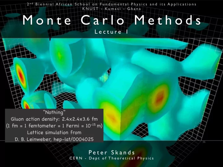
M o n t e C a r l o M e t h o d s L e c t u r e 1 Nothing Gluon - PowerPoint PPT Presentation
2 n d B i e n n i a l A f r i c a n S c h o o l o n F u n d a m e n t a l P h y s i c s a n d i t s A p p l i c a t i o n s K N U S T - K u m a s i - G h a n a M o n t e C a r l o M e t h o d s L e c t u r e 1 Nothing Gluon
2 n d B i e n n i a l A f r i c a n S c h o o l o n F u n d a m e n t a l P h y s i c s a n d i t s A p p l i c a t i o n s K N U S T - K u m a s i - G h a n a M o n t e C a r l o M e t h o d s L e c t u r e 1 “Nothing” Gluon action density: 2.4x2.4x3.6 fm (1 fm = 1 femtometer = 1 Fermi = 10 -15 m) Lattice simulation from D. B. Leinweber, hep-lat/0004025 P e t e r S k a n d s C E R N - D e p t o f T h e o r e t i c a l P h y s i c s
Topics Lecture 1: Numerical Integration + This afternoon Monte Carlo methods Practical Exercises: PYTHIA 8 kickstart Importance Sampling (check the instructions) The Veto Algortihm Lecture 2: Application of these methods to simulations of particle physics: Monte Carlo Event Generators MC Lecture I P. S k a n d s - M o n t e C a r l o m e t h o d s 2
Why Integrals? LHC detector Scattering source Cosmic-Ray detector Neutrino detector Experiments ∆Ω X-ray telescope … → Integrate interaction cross sections over specific regions Predicted number of counts d Ω d σ Z N count ( ∆Ω ) ∝ = integral over solid angle d Ω ∆Ω Differential solid angle element Differential scattering cross section (~ differential scattering probability / MC interaction probability / … ) Lecture I P. S k a n d s - M o n t e C a r l o m e t h o d s 3
Particle Physics Example ALICE : One of the 4 experiments at the Large Hadron Collider at CERN MC More complicated integrals ... Lecture I P. S k a n d s - M o n t e C a r l o m e t h o d s 4
Why Numerical? Let’s look at something simpler … 14 Jun 2000: 4-jet event in ALEPH at LEP (a Higgs candidate) Now compute the backgrounds ... MC Lecture I P. S k a n d s - M o n t e C a r l o m e t h o d s 5
Why Numerical? Part of Z → 4 jets … � � 5.3 Four-parton tree-level antenna functions � 1 1 � 3 12 − 1 � a 0 2 s 12 s 2 34 − 2 s 2 12 s 34 + s 3 2 s 3 ˜ 4 (1 , 3 , 4 , 2) = 34 The tree-level four-parton quark-antiquark antenna contains three final states: quark- s 1234 s 13 s 24 s 134 s 234 4 and ˜ gluon-gluon-antiquark at leading and subleading colour, A 0 A 0 4 and quark-antiquark- 1 3 s 12 s 23 − 3 s 12 s 34 + 4 s 2 12 − s 23 s 34 + s 2 23 + s 2 � � + quark-antiquark for non-identical quark flavours B 0 4 as well as the identical-flavour-only 34 s 13 s 24 s 134 contribution C 0 4 . The quark-antiquark-quark-antiquark final state with identical quark s 3 1 � 1 � 12 2 s 12 s 14 + s 2 + s 13 s 24 ( s 13 + s 23 )( s 14 + s 24 ) + flavours is thus described by the sum of antennae for non-identical flavour and identical- 12 s 13 s 24 ( s 13 + s 23 ) This is one of the simplest processes flavour-only. The antennae for the qgg ¯ q final state are: 1 � 1 � 1 � 3 s 12 + 3 2 s 14 + 3 � 2 s 12 s 23 + s 2 + + 2 s 23 12 … computed at lowest order in the s 13 s 24 ( s 14 + s 24 ) A 0 q ) = a 0 4 (1 , 3 , 4 , 2) + a 0 s 13 s 24 4 (1 q , 3 g , 4 g , 2 ¯ 4 (2 , 4 , 3 , 1) , (5.27) 2 s 3 1 ˜ A 0 a 0 a 0 a 0 a 0 12 4 (1 q , 3 g , 4 g , 2 ¯ q ) = ˜ 4 (1 , 3 , 4 , 2) + ˜ 4 (2 , 4 , 3 , 1) + ˜ 4 (1 , 4 , 3 , 2) + ˜ 4 (2 , 3 , 4 , 1) , (5.28) + [ s 12 s 34 + s 23 s 34 + s 24 s 34 ] + theory. s 13 s 2 s 13 s 134 s 234 ( s 13 + s 23 ) 134 � 1 1 1 a 0 � 2 s 12 s 14 + 2 s 12 s 23 + 2 s 2 12 + s 2 14 + s 2 � 4 (1 , 3 , 4 , 2) = 3 s 12 s 34 − s 24 s 34 − 2 s 2 � � + 23 2 s 13 s 24 s 34 34 s 1234 s 13 s 134 s 234 1 1 s 12 s 24 + s 12 s 34 + 2 s 2 � � + � 3 s 12 s 2 34 − 4 s 2 12 s 34 + 2 s 3 12 − s 3 � + 12 34 s 13 s 134 ( s 13 + s 23 ) 2 s 13 s 24 s 134 s 234 1 1 1 3 s 12 s 23 − 3 s 12 s 34 + 4 s 2 12 − s 23 s 34 + s 2 23 + s 2 � � + Now compute and add the quantum � s 12 s 14 + s 12 s 34 + 2 s 2 � + [ − s 23 − s 24 + 2 s 34 ] + 34 12 s 13 s 24 s 134 s 13 s 134 s 13 s 234 ( s 13 + s 23 ) 3 1 1 + [2 s 12 + s 14 + s 23 ] + [4 s 12 + 3 s 23 + 2 s 24 ] corrections … + [ − 2 s 12 − 2 s 14 + s 24 + 2 s 34 ] 2 s 13 s 24 s 13 s 34 s 13 s 234 1 2 s 3 + [ s 12 s 34 + s 23 s 34 + s 24 s 34 ] 12 s 13 s 2 + 134 s 13 ( s 13 + s 23 )( s 14 + s 24 )( s 13 + s 14 ) 1 � 3 s 12 s 24 + 6 s 12 s 34 − 4 s 2 12 − 3 s 24 s 34 − s 2 24 − 3 s 2 � + 1 s 12 s 24 + 2 s 2 34 � � + s 13 s 134 s 234 12 s 13 ( s 13 + s 23 )( s 13 + s 14 ) 1 + [ − 6 s 12 − 3 s 23 − s 24 + 2 s 34 ] 1 s 12 s 23 + 2 s 2 � � + s 13 s 134 12 s 13 ( s 14 + s 24 )( s 13 + s 14 ) 1 Then maybe worry about � 2 s 12 s 14 + 2 s 12 s 23 + 2 s 2 12 + 2 s 14 s 23 + s 2 14 + s 2 � + s 13 ( s 13 + s 14 ) − 2 2 s 12 1 23 + + [ s 12 + s 23 + s 24 ] s 24 s 34 s 134 s 2 s 13 1 [ − 4 s 12 − s 14 − s 23 + s 34 ] + 1 simulating the detector too … 134 + [ s 12 + 2 s 13 − 2 s 14 − s 34 ] � s 2 1 1 s 24 s 134 34 + [ s 12 − s 34 ] + + O ( � ) . (5.30) 1 − 2 s 12 s 14 s 24 s 134 s 234 s 134 2 s 12 s 2 14 + 2 s 2 14 s 23 + 2 s 2 � � + 14 s 24 s 2 34 s 2 s 2 34 s 134 s 234 134 1 � − 2 s 12 s 14 − 4 s 14 s 24 + 2 s 2 � + 14 s 2 34 s 134 1 − 2 s 12 s 14 − 4 s 2 12 + 2 s 14 s 24 − s 2 14 − s 2 � � + 24 + Additional Subleading Terms … s 34 s 134 s 234 MC 1 1 + [ − 8 s 12 − 2 s 23 − 2 s 24 ] + [ s 12 + s 23 + s 24 ] s 2 s 34 s 134 134 Lecture � 3 1 I + [2 s 12 + s 14 − s 24 − s 34 ] + + O ( � ) (5.29) , 2 s 134 s 234 2 s 134 � � � P. S k a n d s - M o n t e C a r l o m e t h o d s 6
Numerical Integration Problem: find a numerical approximation to the value of S MC Lecture I P. S k a n d s - M o n t e C a r l o m e t h o d s 7
Riemann Sums � b n � f ( x )d x = lim f ( t i )( x i +1 − x i ) n →∞ a i =1 B. Riemann, (1826-1866) MC Lecture I P. S k a n d s - M o n t e C a r l o m e t h o d s 8
Numerical Integration in 1D Fixed-Grid n-point Midpoint (rectangular) Rule: Quadrature Rules Divide into N “bins” of size ∆ Approximate f(x) ≈ constant in each bin Sum over all rectangles inside your region 1 function evaluation per bin MC Lecture I P. S k a n d s - M o n t e C a r l o m e t h o d s 9
Numerical Integration in 1D Fixed-Grid n-point Trapezoidal Rule: Quadrature Rules Approximate f(x) ≈ linear in each bin Sum over all trapeziums inside your region 2 function evaluations per bin MC Lecture I P. S k a n d s - M o n t e C a r l o m e t h o d s 10
Numerical Integration in 1D Fixed-Grid n-point Simpson’s Rule: Quadrature Rules Approximate f(x) ≈ quadratic in each bin Sum over all “Simpsons” inside your region 3 function evaluations per bin MC … and so on for higher n-point rules ... Lecture I P. S k a n d s - M o n t e C a r l o m e t h o d s 11
Convergence Rate The most important question: How long do I have to wait? How many evaluations do I need to calculate for a given precision? Approx Uncertainty n eval / bin Conv. Rate (after n evaluations) (in 1D) Trapezoidal Rule (2-point) 2 1/N 2 Simpson’s Rule (3-point) 3 1/N 4 … m-point (Gauss quadrature) m 1/N 2m-1 See, e.g., F. James, “Monte Carlo See, e.g., Numerical Recipes MC Theory and Practice” Lecture I P. S k a n d s - M o n t e C a r l o m e t h o d s 12
Higher Dimensions Fixed-Grid (Product) Rules scale exponentially with D m-point rule in 1 dimension → m function evaluations per bin 1 2 ... m … in 2 dimensions → m 2 evaluations per bin 2 ... m 2 ... … in D dimensions → m D per bin m E.g., to evaluate a 12-point rule in 10 dimensions , need 1000 billion evaluations per bin MC Lecture I P. S k a n d s - M o n t e C a r l o m e t h o d s 13
Convergence Rate + Convergence is slower in higher Dimensions! → More points for less precision Approx Uncertainty n eval / bin Conv. Rate (after n evaluations) (in D dim) Trapezoidal Rule (2-point) 2 D 1/n 2/D Simpson’s Rule (3-point) 3 D 1/n 4/D … m-point (Gauss rule) m D 1/n (2m-1)/D See, e.g., F. James, “Monte Carlo See, e.g., Numerical Recipes MC Theory and Practice” Lecture I P. S k a n d s - M o n t e C a r l o m e t h o d s 14
A Monte Carlo technique: is any technique making use of random numbers to solve a problem “This risk, that convergence is only given Convergence: with a certain probability, is inherent in Monte Carlo Generators Monte Carlo Generators Monte Carlo Monte Carlo calculations and is the reason Calculus: {A} converges to B why this technique was named after the if an n exists for which world’s most famous gambling casino. |A i>n - B| < ε , for any ε >0 Indeed, the name is doubly appropriate because the style of gambling in the Monte Monte Carlo: {A} converges Carlo casino, not to be confused with the to B if n exists for which noisy and tasteless gambling houses of Las the probability for Vegas and Reno, is serious and | A i>n - B| < ε , for any ε > 0, sophisticated.” is > P , for any P[0<P<1] F. James, “Monte Carlo theory and MC practice”, Rept. Prog. Phys. 43 (1980) 1145 Lecture I P. S k a n d s - M o n t e C a r l o m e t h o d s 15
Recommend
More recommend
Explore More Topics
Stay informed with curated content and fresh updates.
