m = [ 9 ] 1 2 3 4 5 6 7 8 m = [ 1 2 3; 4 5 6; 7 8 9]; m = [ - PDF document

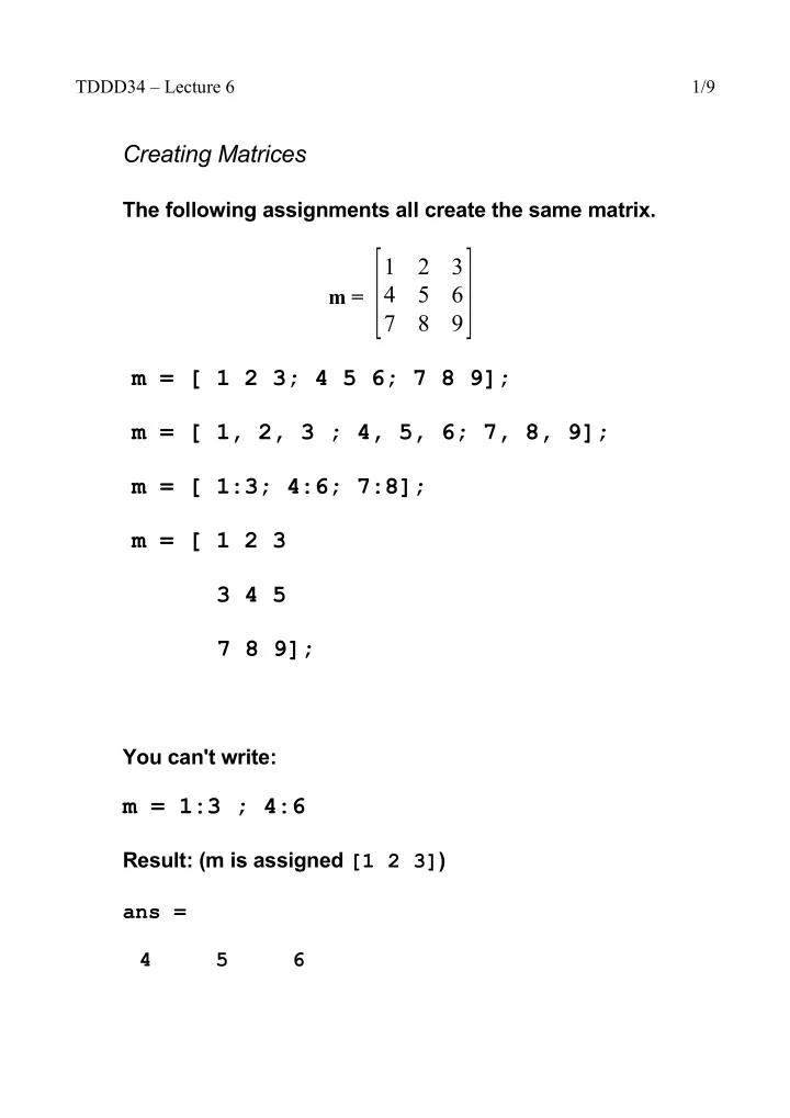
TDDD34 – Lecture 6 1/9 Creating Matrices The following assignments all create the same matrix. m = [ 9 ] 1 2 3 4 5 6 7 8 m = [ 1 2 3; 4 5 6; 7 8 9]; m = [ 1, 2, 3 ; 4, 5, 6; 7, 8, 9]; m = [ 1:3; 4:6; 7:8]; m = [ 1 2 3 3 4 5 7 8 9]; You can't write: m = 1:3 ; 4:6 Result: (m is assigned [1 2 3] ) ans = 4 5 6

TDDD34 – Lecture 6 2/9 z = zeros(5) % produces a 5x5 matrix of zeros o = ones(5) % produces a 5x5 matrix of ones You can also write zeros(5,5) and ones(5,5). You can even have matrices with more dimensions than two. z = zeros(5,5,5)% produces a 5x5x5 matrix of zeros diag can create a diagonal matrix. diag(1:3) => 1 0 0 0 2 0 0 0 3 eye can create an identity matrix. eye(3) => 1 0 0 0 1 0 0 0 1

TDDD34 – Lecture 6 3/9 Some more commands... Transposing: m = m' m = rot90(m) % Rotates m 90 degrees counter- % clockwise m = rot90(m, n) % Rotates m n*90 degrees % counter-clockwise % reshape a matrix reshape(v, rows, columns); reshape(1:5, 5, 1) => 1 2 3 4 5 m = reshape(1:9, 3, 3)' % the same m as before

TDDD34 – Lecture 6 4/9 diag gives a vector with the elements of the diagonal of the matrix m. diag(m) => [1 5 9] You can call sum (or prod ) on a matrix. For example: sum(m) % the m from above. => [12 15 18] Calling sum on a 3-dimensional matrix will give a 2-dimensional matrix and so on. sum(sum(m)) % To calculate the entire sum => 45 % of a 2D matrix. Relational operator works on matrices (of equal dimensions) as well: ~= == < > >= <= When comparing two matrices with these, the result will become a boolean matrix. Once again: the commands any and all become useful.

TDDD34 – Lecture 6 5/9 You can print a matrix with disp . You can calculate the determinant for a certain (square) matrix with the command: det(m) % How are determinants calculated? => 0 Consider the matrix b = [1 2 3 4; 5 6 7 8] l = length(b) => 4 % The largest dimension s = size(b) => [2 4]% [Rows Columns] n = numel(b) => 8 % Number of elements

TDDD34 – Lecture 6 6/9 Just as vectors, matrices can be arguments to functions (like sin, max etc), and can be returned from functions. function m = create_matrix(number) m = round(rand(number) * 10); end plot(m) plots the columns of m versus their index. You can plot a matrix as a color bitmap with the command imagesc. Use this for the ”Game of Life” in lab 6! imagesc(m);

TDDD34 – Lecture 6 7/9 Indexing Matrices m(r, c) % the element of index r (row) and c % (column) in m. Note: If you think in Cartesian Coordiantes this would be equivalent to m(y, x) , not m(x, y) ! m(i, j, k) % Element in a 3-dimensional matrix. You can use vectors to index a matrix: m(2:3, 2:3) => % Rows 2 and 3, Columns 2 and 3 5 6 % from m. 8 9 You can use end to refer to the matrix last column / row. m(end, end) % Element in the lower right corner m(1, 1:end) % The top row of m.

TDDD34 – Lecture 6 8/9 You can put just : instead of an index to select all rows / columns. m(1, :) % The top row of m. m(:, end) % The last column of m. m([1 3:end], :) % Everything in m except row 2 You can concatenate two matrices using brackets: a = [1 2; 3 4] b = [1 0; 0 1] c = [a b] => [1 2 1 0 % Vertical dim. 3 4 0 1] % must ”agree”. d = [a ; b] => [1 2 % Horizontal dim. 3 4 % must ”agree”. 1 0 0 1] You can index a matrix with just one (scalar) index. When doing so, MatLab numbers the elements columnwise. m(3) => 7 % using m from the first m(8) => 6 % slide m(7) => 3

TDDD34 – Lecture 6 9/9 Calculating with Matrices: m1 = [ 1 2 ; 3 4 ; 5 6 ] m2 = m1 * 2; => [ 2 4 ; 6 8 ; 10 12 ] m2 = 2 * m1; => [ 2 4 ; 6 8 ; 10 12 ] m2 = m1 * m1; => ERROR! Why? m2 = m1 * m1'; => [ 5 11 17 ; 11 25 39 ; 17 39 61 ] % How do we calculated this? m2 = m1 .* m1; => [ 1 4 ; 9 16 ; 25 36 ] m2 = m1' * m1; => [ 35 44 ; 44 56 ] We also have the following operators: + - ^ .^ ./ / \ The last two are for matrix left and right-division.