LP Decoding of Regular LDPC Codes in Memoryless Channels Nissim - PowerPoint PPT Presentation
LP Decoding of Regular LDPC Codes in Memoryless Channels Nissim Halabi Guy Even ISIT 2010 1 Low-Density Parity-Check Codes Factor graph representation of LDPC codes: Code C ( G ) and codewords x : x 1 x ( ) ( ) 2 =
LP Decoding of Regular LDPC Codes in Memoryless Channels Nissim Halabi Guy Even ISIT 2010 1
Low-Density Parity-Check Codes Factor graph representation of LDPC codes: Code C ( G ) and codewords x : x 1 x ∑ ( ) ( ) 2 ∈ ⇔ ∀ = C . 0 mod 2 x G c x x c j i 3 1 ( ) ∈ x N c x i j c 4 2 x Local-codes C j = C j ( G ) : 5 c 3 x 6 ∑ ( ) c ∈ ⇔ = x C 0 mod 2 4 x x 7 j i ( ) x c ∈ x N c 8 5 i j x 9 ( d L , d R )- regular LDPC code : x 10 ( ) ∀ ∈ = Variable Check Variables. deg G v v d L nodes nodes ( ) ∀ ∈ = Checks. deg G c c d R (2,4)-regular LDPC code 2
Maximum-Likelihood (ML) Decoding { } { } { } u ∈ k x ∈ n x ∈ n y ∈ ˆ 0,1 0,1 0,1 n Channel MBIOS Channel Encoding Channel Decoding Log-likelihood ratio (LLR) λ i for a received observation y i : ( ) = / 0 y x ( ) λ = / Y X i i ln y i i ( ) = i i / 1 y x / Y X i i i i Any memoryless binary-input output-symmetric (MBIOS) channel can be described by an LLR function. Maximum-likelihood (ML) decoding for any binary-input memory-less channel: ( ) ( ) = λ ML ˆ arg min , x y y x ∈ C x 3
Linear Programming (LP) Decoding Maximum-likelihood (ML) decoding formulated as a linear program: ( ) ( ) ( ) = λ = λ ML ˆ arg min , arg min , x y y x y x ( ) ∈ conv C x ∈ C x C conv( C ) 4
Linear Programming (LP) Decoding Maximum-likelihood (ML) decoding formulated as a linear program: ( ) ( ) ( ) = λ = λ ML ˆ arg min , arg min , x y y x y x ( ) ∈ conv C x ∈ C x Linear Programming (LP) decoding [Fel03, FWK05] – relaxation of the polytope conv( C ) ( ) ( ) = λ LP ˆ arg min , x y y x ∈ C ( ) x conv j check nodes j C conv( C ) conv( C j ) 5
Linear Programming (LP) Decoding Maximum-likelihood (ML) decoding formulated as a linear program: ( ) ( ) ( ) = λ = λ ML ˆ arg min , arg min , x y y x y x ( ) ∈ conv C x ∈ C x Linear Programming (LP) decoding [Fel03, FWK05] – relaxation of the polytope conv( C ) ( ) ( ) = λ LP ˆ arg min , x y y x ∈ C ( ) x conv j check nodes j ˆ LP x integral success! We also know ˆ LP = ˆ ML C (“ML certificate”) x x Solve LP ˆ LP x fractional fail 6
Previous Bounds for LP Decoding (1) No tree assumption! ⇒ Bounds relevant for finite lengths Bounds for specific families of codes: Cycle codes / RA(2) codes over memoryless channels [FK02,HE03]. Expander LDPC codes over bit flipping channels (e.g., BSC, adversarial) [FMSSW04, DDKW07]. Capacity achieving binary expander codes over memoryless channels [FS05]. Non-binary expander codes [Ska09]. 7
Previous Bounds for LP Decoding (2) ( d L , d R ) -regular LDPC codes [KV06, ADS09] - Form of finite length bounds: ∃ c > 1. ∃ t . ∀ noise < t . Pr(LP decoder success) 1 - exp(- c girth ) - If girth = Θ (log n ), then Pr(LP decoder success) 1 - exp(- n γ ), for 0 < γ < 1 n → ∞ : t is a lower bound on the threshold of LP decoding 8
Previous Bounds for LP Decoding (2) ( d L , d R ) -regular LDPC codes [KV06, ADS09] - Form of finite length bounds: ∃ c > 1. ∃ t . ∀ noise < t . Pr(LP decoder success) 1 - exp(- c girth ) - If girth = Θ (log n ), then Pr(LP decoder success) 1 - exp(- n γ ), for 0 < γ < 1 n → ∞ : t is a lower bound on the threshold of LP decoding Koetter and Vontobel ’06 Technique Dual witness technique Memoryless channels Channels BSC( p ) threshold: p LP > 0.01 Example for (3,6)-regular BI-AWGNC( σ ) threshold: LDPC code σ Max-Product = 0.8223 σ LP > 0.5574 E b /N 0 LP < 5.07dB Max-Product ~1.7dB E b / N 0 9
Previous Bounds for LP Decoding (2) ( d L , d R ) -regular LDPC codes [KV06, ADS09] - Form of finite length bounds: ∃ c > 1. ∃ t . ∀ noise < t . Pr(LP decoder success) 1 - exp(- c girth ) - If girth = Θ (log n ), then Pr(LP decoder success) 1 - exp(- n γ ), for 0 < γ < 1 n → ∞ : t is a lower bound on the threshold of LP decoding Koetter and Vontobel ’06 Arora, Daskalakis and Steurer ’09 Technique Dual witness technique Primal LP analysis Memoryless channels BSC Channels BSC( p ) threshold: p LP > 0.01 BSC( p ) threshold: p LP > 0.05 Example for (3,6)-regular p BP = 0.084 BI-AWGNC( σ ) threshold: LDPC code σ Max-Product = 0.8223 σ LP > 0.5574 E b /N 0 LP < 5.07dB Max-Product ~1.7dB E b / N 0 10
Our Results Extension of ADS’09 from BSC to MBIOS channels: Combinatorial characterization: Local Opt. ⇒ LP Opt. Alternative proofs using graph covers [VK05] Finite length bound: decoding errors decrease doubly exponential in the girth of the factor graph Example: for (3,6) -regular LDPC code, σ 0.605 1 3 g 1 4 < ⋅ 2 σ 2 2 P e n c for some constant c < 1 . err 125 Lower bound on thresholds of LP decoding for regular LDPC codes Analytic bounds for MBIOS “Density evolution” bounds on thresholds for BI-AWGNC Example: for (3,6) -regular LDPC code BI-AWGNC( σ ) threshold: σ LP > 0.735 ( σ Max-Product = 0.8223) LP < 2.67dB ( E b / N 0 Max-Product ~1.7dB) E b /N 0 11
Skinny Trees Embedded in Factor Graphs τ , h= 1 Consider a subgraph τ of G: root = v 0 ∈ V L v 0 τ ⊆ Ball( v 0 , 2 h ) ∀ v ∈ τ∩ V L : deg τ ( v ) = deg G ( v ). ∀ c ∈ τ∩ V R : deg τ ( c ) = 2. girth( G ) > 4 h ⇒ τ is a tree – Skinny Tree vars. checks Moreover, in a d L left regular graph d L all skinny trees are isomorphic to: d L -1 d L -1 12
Cost of a Weighted Skinny Tree [ADS09] Given layer weights : → , define -weighted skinny tree τ of height 2h weights ω d L 2 ω 2h d L -1 1 ω 0 Given assignment of LLR values λ to variable nodes, define the cost of an -weighted skinny tree τ − 1 h ( ) ∑ ∑ τ λ ω λ ⋅ , val ω l v = ∈ ∩ τ 0 l v V 2 l 13
Proving Error Bounds using Local Optimality [following ADS09] Local optimality – sufficient condition for the (global) optimality of a decoded codeword based on skinny trees All-Zeros ( ) Assumption < ω ∈ . Then h 1 Theorem: Fix and h girth G + 4 { } { } ( ) ≤ ∃ τ τ λ ≤ = 0 n LP decoding fails skinny tree . , 0 | . val x ω Task: bound the probability that there exists a weighted skinny tree with non-positive cost. 14
Computing [min val ( τ ; λ ) 0] τ – induced graph of factor graph G on Ball( v 0 , 2 h ) { γ } – values associated with variable nodes. – variable nodes of at height 2 l . Y l – check nodes of at height 2 l +1. X l Dyn. Prog. recurrence for computing min cost skinny tree in : = ω γ Basis: leaves: Y 0 0 { } ( ) ( ) − = 1 d 1 Step: checks: min ,..., X Y Y R l l l ( ) ( ) − = ω γ + + + 1 d 1 ... vars: Y X X L − − 1 1 l l l l v 0 X 1 for (3,6)-regular graph , h= 2 15
Computing [min val ( τ ; λ ) 0] τ – induced graph of factor graph G on Ball( v 0 , 2 h ) { γ } – values associated with variable nodes. – variable nodes of at height 2 l . Y l – check nodes of at height 2 l +1. X l Dyn. Prog. recurrence for computing min cost skinny tree in : = ω γ Basis: leaves: Y 0 0 { } ( ) ( ) − = 1 d 1 Step: checks: min ,..., X Y Y R l l l ( ) ( ) − = ω γ + + + 1 d 1 ... vars: Y X X L − − 1 1 l l l l Process: let { γ } = components of LLR v 0 random vector λ . BI-AWGN( σ ) + all zeros assumption: ( ) λ = + φ φ σ 2 1 where . 0, i i i for (3,6)-regular graph , h= 2 16
Density Evolution Based Bound for BI-AWGNC ( σ ) Theorem : Let G denote a ( d L , d R ) -regular bipartite graph with girth Ω (log n ) , and let C ( G ) denote the LDPC code defined by G . Consider the BI-AWGNC( σ ). Then, LP decoding succeeds with probability at least 1 – exp(– n γ ) for some constant 0 < γ < 1 , provided that: R.V. – min cost of a skinny tree with height s (1) s < ¼ girth( G ) , and (2) σ 0 = Lower bound on the Condition (2) holds for σ < σ 0 , where threshold of LP decoding 17
Gaussian PDFs ’ Evolution Probability density functions of X l for l = 0,…,4 ( d L , d R ) = (3,6), and σ = 0.7. = ω γ Y 0 0 { } ( ) ( ) − = 1 1 d min ,..., X Y Y R l l l ( ) ( ) − = ω γ + + + 1 1 d ... Y X X L − − 1 1 l l l l Numeric computation based on quantization following methods used in implementations of density evolution 18
Threshold bound values for finite s , ( d L , d R )=(3,6) σ 0 s E b /N 0 [dB] s = 4 0 0.605 4.36 1 0.635 3.94 2 0.66 3.61 3 0.675 3.41 4 0.685 3.29 6 0.7 3.1 10 0.715 2.91 22 0.735 2.67 Max-Product threshold: σ = 0.82, E b /N 0 ~ 1.7dB 19
Recommend
More recommend
Explore More Topics
Stay informed with curated content and fresh updates.
