Link State Routing Link State Routing Jean-Yves Le Boudec Fall - PDF document
COLE POLYTECHNIQUE FDRALE DE LAUSANNE Link State Routing Link State Routing Jean-Yves Le Boudec Fall 2009 1 Contents Contents 1. Link state flooding topology information finding the shortest paths (Dijkstra) 2. Hierarchical
ÉCOLE POLYTECHNIQUE FÉDÉRALE DE LAUSANNE Link State Routing Link State Routing Jean-Yves Le Boudec Fall 2009 1
Contents Contents 1. Link state flooding topology information finding the shortest paths (Dijkstra) 2. Hierarchical routing with areas 3. OSPF database modelling neighbor discovery - Hello protocol database synchronization link state updates examples 2
1. Link State Routing 1. Link State Routing Pr Prin inciple of link state routing each router keeps a topology database of whole network link state updates flooded, or multicast to all network routers compute their routing tables based on topology often uses Dijkstra’s shortest path algorithm Used in OSPF (Open Shortest Path First), IS-IS (similar to OSPF)and PNNI (ATM routing protocol) 3
(a) Topology Database (a) Topology Database Synchronization Synchronization Neighbouring nodes synchronize before starting any relationship Hello protocol; keep alive initial synchronization of database description of all links (no information yet) Once synchronized, a node accepts link state advertisements contain a sequence number, stored with record in the database only messages with new sequence number are accepted accepted messages are flooded to all neighbours sequence number prevents anomalies (loops or blackholes) 4
Example network Example network � Each router knows directly connected networks n6 n3 B D E n4 n2 n7 n5 A C F n1 5
Initial routing tables Initial routing tables E D net type net type B n6 Ether n6 Ether n7 Ether net type n5 P-to-P n6 n3 n3 Ether n2 P-to-P n4 P-to-P B D E n2 n4 n7 n5 A net type F n1 Ether A C F net type n2 P-to-P n1 Ether C n7 Ether n1 net type n1 Ether n4 P-to-P n5 P-to-P 6
After Flooding After Flooding � The local metric information is flooded to all routers � After convergence, all routers have the same information rtr net cost rtr net cost n6 n3 A n1 10 A n1 10 A n2 100 A n2 100 B n3 10 B n3 10 B D B n2 100 B n2 100 E B n4 100 B n4 100 C n1 10 C n1 10 C n4 100 C n4 100 n2 n4 C n5 100 n7 C n5 100 n5 D n6 10 D n6 10 D n5 100 D n5 100 E n6 10 E n6 10 A C F E n7 10 E n7 10 F n1 10 F n1 10 F n7 10 F n7 10 n1 7
(b) Topology graph (b) Topology graph � Arrows routers-to-nets with a given metric except P-to-P, stub, and external networks � From nets to routers, metric = 0 external network n3 54 0 10 0 100 B D E n6 external 10 stub network network 100 100 0 10 10 n7 0 100 10 100 100 point to point A C F broadcast link network 0 10 10 10 n1 0 0 8
(b) Path Computation (b) Path Computation Performed locally, based on topology database Computes one or several best paths to every destination from this node Best Path = shortest for OSPF OSPF uses Dijkstra’s shortest path the best known algorithm for centralized operation Paths are computed independently at every node synchronization of databases guarantees absence of persistent loops every node computes a shortest path tree root ooted at s ed at self lf 9
Simplified graph Simplified graph � Only arrows with metrics between routers � Every node executes the shortest path computation on the graph – same graph, but different sources 10 B D E 100 100 10 100 10 10 A C F 10 10
Dijkstra’s Shortest Path Algorithm Dijkstra’s Shortest Path Algorithm The nodes are 0...N and the algorithm computes best paths from node 0 c(i,j) is the cost of (i,j) , pred(i) is the predecessor of node i on the tree M being built m(j) is the distance from node 0 to node j . m(0) = 0; M = {0}; m(0) = 0; M = {0}; for k=1 to N { for k=1 to N { find (i0, j0) that minimizes m(i) + c(i,j), find (i0, j0) that minimizes m(i) + c(i,j), with i in M, j not in M with i in M, j not in M m(j0) = m(i0) + c(i0, j0) m(j0) = m(i0) + c(i0, j0) pred(j0) = i0 pred(j0) = i0 M = M ∪ {j0} M = M ∪ {j0} } } as Bellman-Ford, works for any min-plus algebra 11
Example: Dijkstra at A Example: Dijkstra at A init: M = { A } 10 B D E step 1: i0=A 100 100 10 j0=C 100 m(C)=10 M = {A, C} 10 10 A C F m(C)=10 m(A)=0 10 12
Example: Dijkstra at A Example: Dijkstra at A i0=A 10 B D E j0=F m(F)=10 M = {A,C,F} 100 100 10 100 10 10 A C F m(C)=10 m(F)=10 m(A)=0 10 13
Example: Dijkstra at A Example: Dijkstra at A m(F)=20 i0=F 10 B D E j0=E m(E)=20 M = {A,C,F,E} 100 100 10 100 10 10 A C F m(C)=10 m(F)=10 m(A)=0 10 14
Example: Dijkstra at A Example: Dijkstra at A m(D)=30 m(E)=20 i0=E 10 B D E j0=D m(D)=40 M = {A,C,F,E,D} 100 100 10 100 10 10 A C F m(C)=10 m(F)=10 m(A)=0 10 15
Example: Dijkstra at A Example: Dijkstra at A m(D)=30 m(E)=20 m(B)=100 i0=A 10 B D E j0=B m(B)=100 M = {A,C,F,E,D,B} 100 100 10 100 10 10 A C F m(C)=10 m(F)=10 m(A)=0 10 16
Routing table of A Routing table of A A n6 net next n3 n1 direct n2 direct B D n3 B E n4 C n5 C n6 F n2 n4 n7 n5 n7 F A C F n1 17
Test Your Understanding Test Your Understanding Q1: Run Dijkstra at C Q2: What are the routing tables at C solution 18
LS: Summary LS: Summary All nodes compute their own topology database represents the whole network strongly synchronized All nodes compute their best path tree to all destinations Routing tables are built from the tree used for next hop routing only LS versus DV LS avoids convergence problems of DV supports flexible cost definitions; can be used for routing ATM connections LS is much more complex 19
2. Divide large networks 2. Divide large networks Why divide large networks? Cost of computing routing tables update when topology changes SPF algorithm n routers, k links complexity O( n*k ) size of DB, update messages grows with the network size Use hierarchical routing to limit the scope of updates and computational overhead divide the network into several areas independent route computing in each area inject aggregated information on routes into other areas We explain hierarchical routing the OSPF way IS-IS does things a bit differently 20
Hierarchical Routing Hierarchical Routing A large OSPF domain can be configured into areas one backbone area (area 0) non backbone areas (areas numbered other than 0) All inter-area traffic goes through area 0 strict hierarchy Inside one area: link state routing as seen earlier one topology database per area X1 X1 B1 A1 X4 X3 area 1 area 2 X4 X3 B2 A2 area 0 21
Principles Principles Routing method used in the higher level: distance vector no problem with loops - one backbone area Mapping of higher level nodes to lower level nodes area border routers (inter-area routers) belong to both areas Inter-level routing information summary link state advertisements (LSA) from other areas are injected into the local topology databases 22
Example Example Assume networks n1 and n2 become visible at time 0. Show the topology databases at all routers solution X1 X2 6 6 6 n1 10 10 B1 A1 X3 X4 area 1 area 2 10 6 6 10 6 10 X5 X6 B2 A2 10 n2 area 0 23
Hints Hints All routers in area 2 propagate the existence of n1 and n2, directly attached to B1 (resp. B2). Draw the topology database in area 2. Area border routers X4 and X6 belong to area 2, thus they can compute their distances to n1 and n2 Area border routers X4 and X6 inject their distances to n1 and n2 into the area 0 topology database (item 3 of the principle). The corresponding summary link state record is propagated to all routers of area 0. Draw now the topology database in area 0. All routers in area 0 can now compute their distance to n1 and n2, using their distances to X4 and X6, and using the principle of distance vector (item 1 of the principle). Do the computation for X3 and X5. Area border routers X3 and X5 inject their distances to n1 and n2 into the area 1 topology database (item 3 of the principle). Draw now the topology database in area 1. 24
Comments Comments Distance vector computation causes none of the RIP problems strict hierarchy: no loop between areas External and summary LSA for all reachable networks are present in all topology databases of all areas most LSAs are external can be avoided in configuring some areas as terminal: use default entry to the backbone Area partitions require specific support partition of non-backbone area is handled by having the area 0 topology database keep a map of all area connected components partition of backbone cannot be repaired; it must be avoided; can be handled by backup virtual area 0 links through non backbone area 25
*Example of issue : partitioned *Example of issue : partitioned backbone backbone area 0 X1 X2 6 ∞ 6 n1 10 10 B1 A1 X3 X4 area 1 area 2 6 ∞ 10 10 6 10 X5 X6 B2 A2 10 n2 No connectivity between areas via backbone There is a route through Area 2 Virtual link X4 and X6 configure a virtual link through Area 2 virtual link entered into the database, metric = sum of links 26
3. The OSPF Protocol 3. The OSPF Protocol OSPF (Open Shortest Path First) IETF standard for internal routing used in large networks (ISPs) Link State protocol + Hierarchical 27
Recommend
More recommend
Explore More Topics
Stay informed with curated content and fresh updates.
