libadjoint: a new abstraction for developing adjoint models S.W. - - PowerPoint PPT Presentation

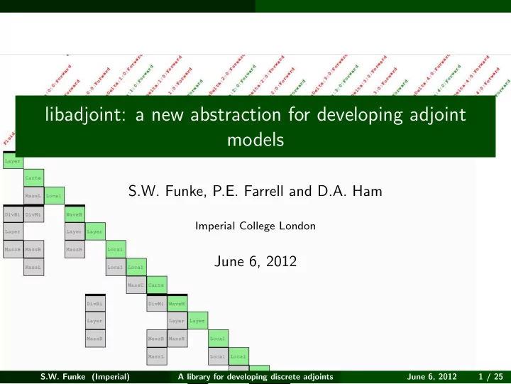
libadjoint: a new abstraction for developing adjoint models

S.W. Funke, P.E. Farrell and D.A. Ham

Imperial College London

June 6, 2012

S.W. Funke (Imperial) A library for developing discrete adjoints June 6, 2012 1 / 25

Outline

Introduction to adjoints Applications Options to adjoin a model Introduction to libadjoint Summary

S.W. Funke (Imperial) A library for developing discrete adjoints June 6, 2012 2 / 25

Introduction to adjoints

Outline

Introduction to adjoints Applications Options to adjoin a model Introduction to libadjoint Summary

S.W. Funke (Imperial) A library for developing discrete adjoints June 6, 2012 3 / 25

Introduction to adjoints

Example problem

What is the optimal turbine layout in a tidal stream to extract most energy from the tidal current?

1

Problem formulation

max

m Power(u, m)

s.t. ut + ∇η = mu, ηt + ∇ · u = 0. m: turbine positions u: velocity η: water elevation. To solve this problem efficiently, we want to apply gradient based

• ptimisation.

How do we compute dPower

dm ?

1Divett et al. Optimisation of multiple turbine arrays in a channel, 2011. S.W. Funke (Imperial) A library for developing discrete adjoints June 6, 2012 4 / 25

Introduction to adjoints

Derivation of the adjoint equation

The general form of the example problem is: min

m J(u, m)

subject to F(u, m) = 0, (1) J(u, m) ∈ R is the functional of interest, m are the control variables and F is the PDE operator with solution u(m).

S.W. Funke (Imperial) A library for developing discrete adjoints June 6, 2012 5 / 25

Introduction to adjoints

Derivation of the adjoint equation

The general form of the example problem is: min

m J(u, m)

subject to F(u, m) = 0, (1) J(u, m) ∈ R is the functional of interest, m are the control variables and F is the PDE operator with solution u(m). We seek the total derivative of J with respect to the controls m: dJ dm = Ju du dm + Jm. (2) Taking the derivative of the constraint in (1) w.r.t. m yields: Fu du dm + Fm = 0. (3)

S.W. Funke (Imperial) A library for developing discrete adjoints June 6, 2012 5 / 25

Introduction to adjoints

Derivation of the adjoint equation

The general form of the example problem is: min

m J(u, m)

subject to F(u, m) = 0, (1) J(u, m) ∈ R is the functional of interest, m are the control variables and F is the PDE operator with solution u(m). We seek the total derivative of J with respect to the controls m: dJ dm = Ju du dm + Jm. (2) Taking the derivative of the constraint in (1) w.r.t. m yields: Fu du dm + Fm = 0. (3) (3) in (2) yields: dJ dm = −

:=λ∗

JuF −1

u Fm + Jm,

where λ is the adjoint solution.

S.W. Funke (Imperial) A library for developing discrete adjoints June 6, 2012 5 / 25

Introduction to adjoints

Adjoint equation

The adjoint equation is therefore: F ∗

u(u, m)λ = J∗ u(u, m)

Key properties

• 1. The adjoint equation is a linear.
• 2. The adjoint equation is solved backward in time.
• 3. The functional gradient is obtained by computing

dJ dm = −λ∗Fm + Jm. Hence the derivative computation requires one forward solve for u and one adjoint solve for λ, independently of the choice of m!

S.W. Funke (Imperial) A library for developing discrete adjoints June 6, 2012 6 / 25

Applications

Outline

Introduction to adjoints Applications Options to adjoin a model Introduction to libadjoint Summary

S.W. Funke (Imperial) A library for developing discrete adjoints June 6, 2012 7 / 25

Applications

Efficient gradient computation

Applications

◮ Sensitivity analysis ◮ Data assimilation ◮ Design optimisation ◮ Inverse problems

S.W. Funke (Imperial) A library for developing discrete adjoints June 6, 2012 8 / 25

Applications

The turbine layout optimisation problem

Figure: Initial and optimised turbine positions and the power increase.

S.W. Funke (Imperial) A library for developing discrete adjoints June 6, 2012 9 / 25

Applications

Goal-oriented adaptivity

Goal-oriented adaptivity

Goal-oriented adaptivity and error control optimises the computational resources by targeting the numerical simulations at a specific quantity of interest.

2

• 2W. Bangerth, R. Rannacher. Adaptive Finite Element Methods for

Differential Equations, 2003.

S.W. Funke (Imperial) A library for developing discrete adjoints June 6, 2012 10 / 25

Options to adjoin a model

Outline

Introduction to adjoints Applications Options to adjoin a model Introduction to libadjoint Summary

S.W. Funke (Imperial) A library for developing discrete adjoints June 6, 2012 11 / 25

Options to adjoin a model

The stages of developing a model

Continuous equations Discretised equations Source code

S.W. Funke (Imperial) A library for developing discrete adjoints June 6, 2012 12 / 25

Options to adjoin a model

Continuous adjoint

Continuous adjoint Continuous equations Discretised equations Source code pen+paper

S.W. Funke (Imperial) A library for developing discrete adjoints June 6, 2012 13 / 25

Options to adjoin a model

Algorithmic differentiation

Continuous adjoint Continuous equations Discretised equations Source code Adjoint of the source code automatic differentiation tool pen+paper

S.W. Funke (Imperial) A library for developing discrete adjoints June 6, 2012 14 / 25

Options to adjoin a model

Libadjoint’s approach

Continuous adjoint Continuous equations Discretised equations Source code Adjoint of the source code automatic differentiation tool pen+paper Adjoint of the discretised equations libadjoint

S.W. Funke (Imperial) A library for developing discrete adjoints June 6, 2012 15 / 25

Introduction to libadjoint

Outline

Introduction to adjoints Applications Options to adjoin a model Introduction to libadjoint Summary

S.W. Funke (Imperial) A library for developing discrete adjoints June 6, 2012 16 / 25

Introduction to libadjoint

The fundamental idea of Libadjoint

libadjoint is a library that facilitates the development of discrete adjoint models.

The fundamental idea of AD

A model is a sequence of elementary instructions.

S.W. Funke (Imperial) A library for developing discrete adjoints June 6, 2012 17 / 25

Introduction to libadjoint

The fundamental idea of Libadjoint

libadjoint is a library that facilitates the development of discrete adjoint models.

The fundamental idea of AD

A model is a sequence of elementary instructions.

The fundamental idea of libadjoint

A model is a sequence of equation solves.

S.W. Funke (Imperial) A library for developing discrete adjoints June 6, 2012 17 / 25

Introduction to libadjoint

Example: Burgers equation

The non-viscous Burgers equation has the form: ∂u ∂t + u · ∇u = 0. The (explicit) discretisation with one nonlinear iteration per time step yields: −(M + ∆tA(un))

• :=T(un)

un + Mun+1 = 0, where M is the mass matrix, A is the discretised advection operator and ∆t is the time step. We linearise the advection term using the velocity at the previous time step.

S.W. Funke (Imperial) A library for developing discrete adjoints June 6, 2012 18 / 25

Introduction to libadjoint

Example: Burgers equation

Three time steps can be written as a block matrix:

    I T (u0) M T (u1) M T (u2) M    

• F (u)

    u0 u1 u2 u3    

u

=     uinit    

• b

We have cast the model in the form F(u)u = b.

S.W. Funke (Imperial) A library for developing discrete adjoints June 6, 2012 19 / 25

Introduction to libadjoint

Example: Burgers equation

Three time steps can be written as a block matrix:

    I T (u0) M T (u1) M T (u2) M    

• F (u)

    u0 u1 u2 u3    

u

=     uinit    

• b

We have cast the model in the form F(u)u = b. The associated adjoint equation is:

• F(u) + ∂F(u)

∂u u ∗ λ = ∂J ∂u

∗

.

S.W. Funke (Imperial) A library for developing discrete adjoints June 6, 2012 19 / 25

Introduction to libadjoint

Example: Burgers equation

Three time steps can be written as a block matrix:

    I T (u0) M T (u1) M T (u2) M    

• F (u)

    u0 u1 u2 u3    

u

=     uinit    

• b

We have cast the model in the form F(u)u = b. The associated adjoint equation is:

• F(u) + ∂F(u)

∂u u ∗ λ = ∂J ∂u

∗

. Therefore the adjoint equation reads:

         I∗

• T (u0) + ∂T (u0)

∂u0

u0 ∗ M∗

• T (u1) + ∂T (u1)

∂u1

u1 ∗ M∗

• T (u2) + ∂T (u2)

∂u2

u2 ∗ M∗              λ0 λ1 λ2 λ3     = ∂J ∂u

∗

. S.W. Funke (Imperial) A library for developing discrete adjoints June 6, 2012 19 / 25

Introduction to libadjoint

The development of an adjoint model with libadjoint requires two steps:

• 1. Annotation
• 2. Callback registration

S.W. Funke (Imperial) A library for developing discrete adjoints June 6, 2012 20 / 25

Introduction to libadjoint

Step 1: Annotation

◮ libadjoint provides a set of library calls with which a model may be

annotated at runtime

◮ Each equation solve is annotated to record what is being computed,

what operators are acting on previously computed values, and their nonlinear dependencies

The annotation

is sufficient to describe the discretisation matrix of the forward model...

    I T(u0) M T(u1) M T(u2) M    

S.W. Funke (Imperial) A library for developing discrete adjoints June 6, 2012 21 / 25

Introduction to libadjoint

Step 1: Annotation

...and so libadjoint can derive the associated adjoint system:

S.W. Funke (Imperial) A library for developing discrete adjoints June 6, 2012 22 / 25

Introduction to libadjoint

Step 2. Register function callbacks

◮ libadjoint offers the facility to register function callbacks for

computing the action of the operators in the annotation

◮ ... and their derivatives (e.g. by using AD) ◮ It also offers the facility to record solutions

With the callbacks ...

... libadjoint can automatically assemble the adjoint equations.

S.W. Funke (Imperial) A library for developing discrete adjoints June 6, 2012 23 / 25

Introduction to libadjoint

Key properties of libadjoint

+ Works with modern language features and external libraries + The approach meshes well with AD + Comes with an optimal checkpointing strategy: Revolve3 − The annotation and callback implementation has to be done by hand, however in some cases this can be automated (DOLFIN)

• 3A. Griewank, A. Walther, Revolve: an implementation of checkpointing for

the reverse or adjoint mode of computational differentiation, TOMS (2000)

S.W. Funke (Imperial) A library for developing discrete adjoints June 6, 2012 24 / 25

Summary

Summary

We have seen:

◮ An introduction and applications to adjoints ◮ Three ways how to adjoint a model ◮ How to adjoint a model using libadjoint

S.W. Funke (Imperial) A library for developing discrete adjoints June 6, 2012 25 / 25