LECTURES ON STATISTICS AND DATA ANALYSIS Columbia University, June - PowerPoint PPT Presentation

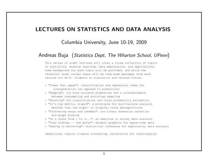
LECTURES ON STATISTICS AND DATA ANALYSIS Columbia University, June 10-19, 2009 Andreas Buja ( Statistics Dept, The Wharton School, UPenn ) This series of eight lectures will cover a loose collection of topics in statistics, machine learning, data exploration, and applications. Some background for each topic will be provided, and while the technical level varies there will be take-home messages from each lecture for Ph.D. students in statistics and related fields. * "Trees that speak": classification and regression trees for interpretation (as opposed to prediction) * "Bagging", its bias-variance properties and a correspondence between subsampling and bootstrap sampling * "Boosting" for classification and class probability estimation * "It’s the metric, stupid": a principle for multivariate analysis methods that use eigen- or singular value decompositions * "Flattening warps and cobwebs": non-linear dimension reduction and graph drawing * "On a scale from 1 to 3...": an exercise in survey data analysis * "Tuna fishing -- the movie": dynamic graphics for space-time data * "Seeing is believing": statistical inference for exploratory data analysis (Additional topics: k-means clustering, calibration for simultaneity) 1

Some Bio • PhD 1980 from ETH (Zurich, Switzerland) in Statistics/Math • -1981 Children’s Hospital (Zurich) & ETH • -1982 Visiting Asst Prof Stanford U & SLAC • -1985 Asst Prof, U of Wash, Seattle • 1986 Visiting Bellcore (J. Kettenring, R. Gnanadesikan) • 1987 Salomon Brothers (4 months) • -1994 Bellcore • -1995 AT&T Bell Labs (D. Pregibon, D. Lambert) • -2001 AT&T Labs • -present: The Wharton School, UPenn, Philadelphia 2

FIRST TOPIC: EXPLORING THE UNIVERSE OF LOSS FUNCTIONS FOR CLASS PROBABILITY ESTIMATION JoinL Work with Werner Stuetzle ( Statistics Dept, University of Washington ) Yi Shen ( then at Wharton ) (Part of the work done while AB and WS were with AT&T Labs ) 3

Example • Data: AT&T Labs’ store of call detail records • Problem: Find residences with home businesses • Idea: Look for phone numbers with calling patterns that resemble those of small businesses • Training data: Several months of calls of 50K small businesses and 50K residences • Feature extraction: > 100 counts such as # { calls: weekdays, 9am < begin < 11am, 1min < dur < 10min } • Techniques: Boosting vs. logistic ridge regression • Use: Scoring of > 50,000,000 residences score = ˆ P (small business) 4

Coefficients of Logistic Ridge Regression Red => business-likeness, Blue => residence-likeness Weekdays Weekends 1 1 1 2 1 1 1 2 9 2 3 7 0 2 9 2 3 7 0 2 6 - - - - - 3 6 - - - - - 3 1 1 1 2 2 1 1 1 2 2 - - - - 9 2 3 7 0 3 6 9 2 3 7 0 3 6 Term=Res. Term=Res. <1m <1m 1m-10m 1m-10m >10m >10m 1 1 1 2 1 1 1 2 9 2 3 7 0 2 9 2 3 7 0 2 6 - - - - - 3 6 - - - - - 3 1 1 1 2 2 1 1 1 2 2 - - - - 9 2 3 7 0 3 6 9 2 3 7 0 3 6 Term=Biz. Term=Biz. <1m <1m 1m-10m 1m-10m >10m >10m Term. = Unknown Term. = Unknown 1 1 1 2 1 1 1 2 9 2 3 7 0 2 9 2 3 7 0 2 6 - - - - - 3 6 - - - - - 3 1 1 1 2 2 1 1 1 2 2 - - - - 9 2 3 7 0 3 6 9 2 3 7 0 3 6 <1m <1m 1m-10m 1m-10m >10m >10m 5

Conclusions from the Example: • Classification is sometimes not sufficient. • Real interest: Class Probability Estimation • “Labeled data” can be available if looked at the right way • Rich bag of tools: Discriminant analysis, logistic regression, boosting, SVMs, CART, random forests, ... • ... but class probability estimation takes a back seat to classification. 6

Basics 1: Learning/Classification • Supervised vs unsupervised classification • Binary vs multi-class classification • Training data: ( x n , y n ) , n = 1 ...N R K : • x n ∈ I features, predictors • y n ∈ { 0 , 1 } : class labels, responses 7

Basics 2: Stochastics • Assumption intuitively: sampling • Assumption, technically: ( x n , y n ) i.i.d. realizations of ( X , Y ) – Marginal distribution of predictors: f ( x ) = P [ d x ] /d x – Conditional distribution of labels: η ( x ) = P [ Y = 1 | X = x ] = E [ Y | X = x ] Together they describe the joint distribution of X and Y : P [ Y = 1 , d x ] = P [ Y = 1 | X = x ] P [ d x ] = η ( x ) f ( x ) d x 8

Basics 3: Classification vs Class Prob Estimation • Classifier cl( x ) : cl( x ) = cl( x ; ( x n , y n ) n =1 ...N ) ∈ { 0 , 1 } • Class probability estimator p ( x ) : p ( x ) = p ( x ; ( x n , y n ) n =1 ...N ) ∈ [0 , 1] • Class probability estimators define classifiers: p ( x ) �→ cl( x ) cl( x ) = 1 [ p ( x ) >t ] (e.g. t = 0 . 5 ) • Estimation: p ( x ) estimates η ( x ) , cl( x ) estimates 1 η ( x ) >t . • (Note on ML history: Early ML assumed classes to be perfectly separable: η ( x ) = 1 A ( x ) . ⇒ No distinction between classification and class prob estimation. ⇒ Classification is a purely geometric problem of finding boundaries. ) 9

Basics 4: Differences in Conventions between ML and Stats • Notation: Relabeling of classes {− 1 , +1 } ↔ { 0 , 1 } y ∗ = 2 y − 1 • ± 1 response vs 0-1 response: cl ∗ ( x ) = 2 cl( x ) − 1 • ± 1 classifier vs 0-1 classifier: y ∗ cl ∗ ( x ) = 1 • ( x , y ) is correctly classified iff: cl ∗ ( x ) = +1 cl ∗ ( x ) = − 1 Product y ∗ = +1 − 1 +1 y ∗ = − 1 − 1 +1 • Misclassification rate := P [ y � = cl] = P [ y ∗ cl ∗ = − 1] What assumption was made in this definition? (Diabetics ...) 10

Basics 5: Quantile Classification and Unequal Cost Classification • Common in older AI/ML work: Equal misclassification cost for ⇒ y = 0 , cl = 1 false positive y = 1 , cl = 0 ⇒ false negative • Assume cost c ∈ (0 , 1) for misclassifying y = 0 as cl = 1 (false positive) 1 − c and cost for misclassifying y = 1 as cl = 0 (false negative) � c when y = 0 , cl = 1 � L ( y | cl) = = y (1 − c )1 cl=0 + (1 − y ) c 1 cl=1 1 − c when y = 1 , cl = 0 • Local/pointwise Risk = E [ L ( Y | cl)] =: L ( η | cl) when P [ Y = 1] = η : � (1 − η ) c when cl = 1 � L ( η | cl) = = η (1 − c )1 cl=0 + (1 − η ) c 1 cl=1 η (1 − c ) when cl = 0 11

Basics 5 (contd.): Quantile Classification and Unequal Cost Classification • Bayes Risk = min cl ∈{ 0 , 1 } L ( η | cl) = min( (1 − η ) c, η (1 − c ) ) • Minimizer: Classify cl = 1 when η > c 1 1 cl=0: η → η (1−c) 1−c Risk cl=1: η → ( 1 − η ) c c Bayes Risk( η ) 0 0 0 c 1 η 12

Basics 5 (contd.): Quantile Classification and Unequal Cost Classification • Equivalence: - classification at quantile c and - classification with costs c/ (1 − c ) for false positives/negatives In particular: Median classification = Equal-cost classification • Population Bayes risk: If we knew η ( X ) , the average Bayes risk would be E [ min( (1 − η ( X )) c, η ( X ) (1 − c ) )] = unavoidable average misclassification cost • Baseline misclassification rate: If η 1 = P [ Y = 1] = E [ η ( X )] is the marginal class 1 probability, then the trivial classifier that ignores X is cl = 1 if η 1 > c and cl = 0 otherwise. Any classifier that uses predictors X must beat the baseline classifier min( (1 − η 1 ) c, η 1 (1 − c ) ) . with risk 13

Basics 6: Statisticians’ True and Trusted Tools • Logistic regression : a conditional model of Y given X η ( x ) = ψ ( x ′ β ) , ψ ( F ) = 1 / (1 + exp( − F )) Idea: Estimate a linear model and map the values to the range (0,1). • Linear discriminant analysis (LDA): a conditional model of X given Y f ( X | Y = 1) ∼ N ( µ 1 , Σ) , f ( X | Y = 0) ∼ N ( µ 0 , Σ) Actually, this is equivalent to LS regression of the 0-1 response Y on X . • Extensions to more than two classes exist: multinomial logistic regression and multi-class discriminant analysis. • Non-parametric extensions exist: . logistic regression with polynomial or spline bases, ... . LDA based on non-linear transformations of X : FDA (Hastie et al. 94) 14

Basics 7: Recap of Logistic Regression F ( x ) = x ′ β • Logistic link and linear model: η ( x ) = ψ ( F ( x )) , ψ ( F ) = 1 / (1 + e − F ) , Logit ( η ) = log( η/ (1 − η )) , 1 − ψ ( F ) = ψ ( − F ) • Loss from one observation when observing y ∈ { 0 , 1 } and guessing ˆ η = p : L ( y | p ) = − log likelihood of a Bernoulli variable − log( p y (1 − p ) 1 − y ) = − y log( p ) − (1 − y ) log(1 − p ) = � − log( p ) when y =1 � = ≥ 0 − log(1 − p ) when y =0 F = x ′ β • Composed for one observation ( x , y ) : log(1 + e − y ∗ F ) − log( ψ ( y ∗ F )) = L ( y | ψ ( F )) = F n = x ′ • Composed for a sample ( x n , y n ) , n = 1 ...N : n β , p n = ψ ( F n ) n =1 ,...,N L ( y n | ψ ( x ′ n =1 ,...,N log(1 + e − y ∗ n F n ) � n β )) = � 15