Lecture 7: Game theory David Aldous February 24, 2016 STAT 155 is - PowerPoint PPT Presentation
Lecture 7: Game theory David Aldous February 24, 2016 STAT 155 is an entire course on Game Theory. In this lecture we illustrate Game Theory by first focusing on one particular game for which we can get data. The game is relevant to one of the
Lecture 7: Game theory David Aldous February 24, 2016
STAT 155 is an entire course on Game Theory. In this lecture we illustrate Game Theory by first focusing on one particular game for which we can get data. The game is relevant to one of the central ideas of game theory, Does the data – how people actually play the game – correspond roughly to what theory says? We will do some math calculations “because we can” – more details in write-up. Continuing to analyze the data, or doing a simulation study of more complex strategies, would be a nice course project . Also, finding and studying some other observable online game-theoretic game wold be a good project. There are many introductory textbooks and less technical accounts of game theory – see write-up. Here is a 1-slide overview.
Setting: players each separately choose from a menu of actions, and 1 get a payoff depending (in a known way) on all players’ actions. Rock-paper-scissors illustrates that one should use a randomized 2 strategy, and so we assume a player’s goal is to maximize their expected payoff. There is a complete theory of such two-person zero-sum games. For other games, a fundamental concept is Nash equilibrium 3 strategy: one such that, if all other players play that strategy, then you cannot do better by choosing some other strategy. This concept is motivated by the idea that, if players adjust their strategies in a selfish way, then strategies will typically converge to some Nash equilibrium. More advanced theory is often devoted to settings where Nash 4 equilibria are undesirable in some sense, as with Prisoners’ Dilemma, and to understanding why human behavior is not always selfish.
A (slightly simplified) math description of the actual game we shall study. There are 5 items of somewhat different known values, say { 8 , 7 , 6 , 5 , 4 } dollars. There are 10 players. A player can make a sealed bid for (only) one item, during a window of time. During the time window, players see how many bids have already been placed on each item, but do not see the bid amounts. When time expires each item is awarded to the highest bidder on that item. We assume players are seeking to maximize their expected gain. So a player has to decide three things; when to bid, which item to bid on, and how much to bid.
The game is called Dice City Roller on pogo.com . [show DCR in progress] We get data by screenshots at 14, 5 and 0 seconds before deadline, and then after winning bids are shown. Who are the actual players? [show profiles]
We study math for simplified version without the time window – each player just places a sealed bid without knowledge of other players actions. In this case we can calculate the Nash equilibrium strategy explicitly – for any number of players, and any number and values of items. Start with the simplest setting: 2 players, 2 items of values 1 and b , where 0 < b ≤ 1. We have a little data from playing this in Lecture 1. [show data] [show bidding-analysis] and the winner of the Lecture 1 game is . . . . . .
[2014] 24/35 students bid on the $1, 11/35 bid on the 50c bids on $1 bids on 50c 0 0 0 25 1 41 10 42 25 45 26 48 32 49 49 49 49 49 49 37 50 50 50 50 40 51 45 55 49 67 75 75 80 81 100 Consider a person P who bid 49. When we match with a random other person: chance 12/34 P gains 0 (other person bid more on the $1) chance 17/34 P gains 51 (= 100 - 49) (P won the bid) chance 5/34 we do coin-toss to decide winner: P gains 51/2. So P's expected gain = 29.25 ______________________________________________________________________ [2016] 18/35 students bid on the $1, 17/35 bid on the 50c bids on $1 bids on 50c 20 1 1 50 50 50 50 50 2 62 5 65 10 70 70 70 30 30 74 38 75 75 40 40 76 45 45 83 48 48 48 95 50 50 99
I will develop some math theory, first in this “two players, two items” setting. My point is to show that it’s not terribly complicated. See write-up for more theory.
A player’s strategy is a pair of functions ( F 1 , F b ): F 1 ( x ) = P ( bid an amount ≤ x on the first item) , 0 ≤ x ≤ 1 (1) F b ( y ) = P ( bid an amount ≤ y on the second item) , 0 ≤ y ≤ b (2) where F 1 (1) + F b ( b ) = 1 . (3) We can equivalently work with the associated densities f 1 ( x ) = F ′ 1 ( x ) , f b ( y ) = F ′ b ( y ) . Suppose your opponent’s strategy is some function ( f 1 , f b ) and your strategy is some function ( g 1 , g b ). What is the formula for your expected gain? [do on board]
opponent’s strategy is ( f 1 , f b ), your strategy is ( g 1 , g b ). Your expected gain is � 1 � b (1 − x ) g 1 ( x )[ F 1 ( x )+ F b ( b )] dx + ( b − y ) g b ( y )[ F b ( y )+ F 1 (1)] dy . (4) 0 0 We need an obvious fact [picture on board]. Given a payoff function h ( x ) ≥ 0 with h ∗ = max x h ( x ), consider the � expected payoff h ( x ) g ( x ) dx when we choose x according to a probability density g . Then we get the maximum expected payoff if and only if h ( x ) = c for all x ∈ support( g ) h ( x ) ≤ c for all x �∈ support( g ) for some c (which is in fact h ∗ ). Now our expected gain (4) is of this form, thinking of ( g 1 , g b ) as a single probability density function. Apply the “obvious fact”:
So given your opponent’s strategy ( f 1 , f b ), your expected gain is maximized by choosing a strategy ( g 1 , g b ) satisfying, for some constant c (1 − x )[ F 1 ( x ) + F b ( b )] = c on support( g 1 ) ≤ c off support( g 1 ) ( b − y )[ F b ( y ) + F 1 (1)] = c on support( g b ) ≤ c off support( g b ) Now the definition of ( f 1 , f b ) being a Nash equilibrium strategy is precisely the assertion that (5 - 8) hold for ( g 1 , g b ) = ( f 1 , f b ). So now we have a set of equations for the NE strategy.
(1 − x )[ F 1 ( x ) + F b ( b )] = c on support( f 1 ) (5) ≤ c off support( f 1 ) (6) ( b − y )[ F b ( y ) + F 1 (1)] = c on support( f b ) (7) ≤ c off support( f b ) (8) with “boundary conditions” F 1 (0) = F b (0) = 0; F 1 (1) + F b ( b ) = 1 . Note that in any game we can do some similar argument to get equations that a NE must satisfy. STAT 155, like most game theory, focusses on a discrete menu of actions – our example is continuous. Theory talks about existence and uniqueness of solutions, for general games. We can just go ahead and solve these particular equations. The write-up shows how to solve “as math” without thinking about the game interpretation. The answer appears as
b 1 1 F 1 ( x ) = 1+ b ( 1 − x − 1) on 0 ≤ x ≤ (9) 1+ b b 2 1 b F b ( y ) = 1+ b ( b − y − 1) on 0 ≤ y ≤ 1+ b . (10) The corresponding densities are 1+ b (1 − x ) − 2 on 0 ≤ x ≤ b 1 f 1 ( x ) = (11) 1+ b 1+ b ( b − y ) − 2 on 0 ≤ y ≤ b 2 b f b ( y ) = 1+ b . (12) [show figure] The expected gain for each player works out as b E [ gain ] = 1 + b .
An important general principle If opponents play the NE strategy then any non-random choice of action you make in the support of the NE strategy will give you the same expected gain (which equals the expected gain if you play the random NE strategy), and any other choice will give you smaller expected gain. This “ constant expected gain ” principle is true because the NE expected gain is an average gain over the different choices in its support; if these gains were not constant then one would be larger than the NE gain, contradicting the definition of NE. In our game, if you bid x on item 1, where x is in the support 1 0 ≤ x ≤ 1+ b , then your chance of winning is (by calculation) 1+ b (1 − x ) − 1 = 1+ b (1 − x ) − 1 , so your expected gain is (1 − x ) × b b b 1+ b as the general principle says. Later we will use the general principle to calculate the NE for arbitrary numbers of players and prizes.
Note that the gap between your maximum bid and the item’s value is the same for both items; 1 − 1 / (1 + b ) = b − b 2 / (1 + b ) = b / (1 + b ) . This follows from the “constant expected gain” principle above; if you bid the maximum value in the support the you are certain to win the item, so your gain must be the same for both items. The same “equal gap principle” works by the same argument for general numbers of players and items (but is special to our particular game). [show figure – how close is data to theory?]
Consider the general case of N ≥ 2 players and M ≥ 2 items of values b 1 ≥ b 2 ≥ . . . ≥ b M > 0. The bottom line (with a side condition I’ll explain) is the formula � N − 1 � M − 1 E ( gain to a player at NE) = c = (13) i b − 1 / ( N − 1) � i and the NE strategy is defined by the density functions f i ( x ) = M − 1 1 ( b i − x ) − N / ( N − 1) , 0 ≤ x ≤ b i − c N − 1 j b − 1 / ( N − 1) � j for bids on prize i . The next slide shows the main steps in the calculation.
Writing out the expression for the expected gain when you bid x i on the i ’th item, the “constant expected gain” property says i ) − F i ( x ))) N − 1 = c , ( b i − x ) (1 − ( F i ( x ∗ 0 ≤ x ≤ x ∗ i := b i − c (14) where c = expected gain to a player at NE. Because a strategy is a probability distribution we have � i F i ( x ∗ i ) = 1 and so � (1 − F i ( x ∗ i )) = M − 1 . i Now using (14) with x = 0 we have i ) = ( c / b i ) 1 / ( N − 1) 1 − F i ( x ∗ (15) and so ( c / b i ) 1 / ( N − 1) = M − 1 � i identifying c .
Recommend
More recommend
Explore More Topics
Stay informed with curated content and fresh updates.


