Lecture 03: Duration Calculus I 2014-05-08 Dr. Bernd Westphal 03 - PowerPoint PPT Presentation
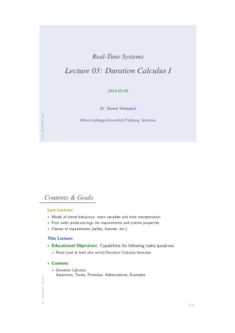
Real-Time Systems Lecture 03: Duration Calculus I 2014-05-08 Dr. Bernd Westphal 03 2014-05-08 main Albert-Ludwigs-Universit at Freiburg, Germany Contents & Goals Last Lecture: Model of timed behaviour: state
Real-Time Systems Lecture 03: Duration Calculus I 2014-05-08 Dr. Bernd Westphal – 03 – 2014-05-08 – main – Albert-Ludwigs-Universit¨ at Freiburg, Germany
Contents & Goals Last Lecture: • Model of timed behaviour: state variables and their interpretation • First order predicate-logic for requirements and system properties • Classes of requirements (safety, liveness, etc.) This Lecture: • Educational Objectives: Capabilities for following tasks/questions. • Read (and at best also write) Duration Calculus formulae. • Content: • Duration Calculus: Assertions, Terms, Formulae, Abbreviations, Examples – 03 – 2014-05-08 – Sprelim – 2 /33
Duration Calculus – 03 – 2014-05-08 – main – 3 /33
Duration Calculus: Preview gas valve flame sensor • Duration Calculus is an interval logic . • Formulae are evaluated in an ignition ( implicitly given ) interval. • G, F, I, H : { 0 , 1 } Strangest operators : • Define L : { 0 , 1 } as G ∧¬ F . • everywhere — Example: ⌈ G ⌉ (Holds in a given interval [ b, e ] iff the gas valve is open almost everywhere.) • chop — Example: ( ⌈¬ I ⌉ ; ⌈ I ⌉ ; ⌈¬ I ⌉ ) = ⇒ ℓ ≥ 1 (Ignition phases last at least one time unit.) – 03 – 2014-05-08 – Sdcpreview – ℓ • integral — Example: ℓ ≥ 60 = ⇒ ∫ L ≤ 20 (At most 5% leakage time within intervals of at least 60 time units.) 4 /33
Duration Calculus: Overview We will introduce three (or five) syntactical “levels”: (i) Symbols: f, g, true , false , = , <, >, ≤ , ≥ , x, y, z, X, Y, Z, d (ii) State Assertions: P ::= 0 | 1 | X = d | ¬ P 1 | P 1 ∧ P 2 (iii) Terms: θ ::= x | ℓ | ∫ P | f ( θ 1 , . . . , θ n ) (iv) Formulae: – 03 – 2014-05-08 – Sdcpreview – F ::= p ( θ 1 , . . . , θ n ) | ¬ F 1 | F 1 ∧ F 2 | ∀ x • F 1 | F 1 ; F 2 (v) Abbreviations: ⌈ P ⌉ t , ⌈ P ⌉ ≤ t , ⌈ ⌉ , ⌈ P ⌉ , ♦ F, � F 5 /33
Symbols: Syntax • f, g : function symbols , each with arity n ∈ N 0 . Called constant if n = 0 . Assume: constants 0 , 1 , · · · ∈ N 0 ; binary ‘ + ’ and ‘ · ’. • p, q : predicate symbols , also with arity. Assume: constants true , false ; binary = , <, >, ≤ , ≥ . • x, y, z ∈ GVar: global variables . • X, Y, Z ∈ Obs: state variables or observables , each of a data type D (or D ( X ) , D ( Y ) , D ( Z ) to be precise). – 03 – 2014-05-08 – Sdcsymb – Called boolean observable if data type is { 0 , 1 } . • d : elements taken from data types D of observables. 6 /33
Symbols: Semantics • Semantical domains are • the truth values B = { tt , ff } , • the real numbers R , • time Time, (mostly Time = R + 0 (continuous), exception Time = N 0 (discrete time)) • and data types D . • The semantics of an n -ary function symbol f is a (mathematical) function from R n to R , denoted ˆ f , i.e. f : R n → R . ˆ – 03 – 2014-05-08 – Sdcsymb – • The semantics of an n -ary predicate symbol p is a function from R n to B , denoted ˆ p , i.e. p : R n → B . ˆ 7 /33
Symbols: Examples • The semantics of the function and predicate symbols assumed above is fixed throughout the lecture: ˆ ˆ • true = tt, false = ff • ˆ 0 ∈ R is the (real) number zero , etc. + : R 2 → R is the addition of real numbers, etc. • ˆ = : R 2 → B is the equality relation on real numbers, • ˆ < : R 2 → B is the less-than relation on real numbers, etc. • ˆ – 03 – 2014-05-08 – Sdcsymb – • “Since the semantics is the expected one, we shall often simply use the symbols 0 , 1 , + , · , = , < when we mean their semantics ˆ 0 , ˆ 1 , ˆ = , ˆ + , ˆ · , ˆ < .” 8 /33
Symbols: Semantics • The semantics of a global variable is not fixed (throughout the lecture) but given by a valuation , i.e. a mapping V : GVar → R assigning each global variable x ∈ GVar a real number V ( x ) ∈ R . We use Val to denote the set of all valuations, i.e. Val = ( GVar → R ) . Global variables are though fixed over time in system evolutions. – 03 – 2014-05-08 – Sdcsymb – 9 /33
Symbols: Semantics • The semantics of a global variable is not fixed (throughout the lecture) but given by a valuation , i.e. a mapping V : GVar → R assigning each global variable x ∈ GVar a real number V ( x ) ∈ R . We use Val to denote the set of all valuations, i.e. Val = ( GVar → R ) . Global variables are though fixed over time in system evolutions. • The semantics of a state variable is time-dependent . It is given by an interpretation I , i.e. a mapping I : Obs → ( Time → D ) – 03 – 2014-05-08 – Sdcsymb – assigning each state variable X ∈ Obs a function I ( X ) : Time → D ( X ) such that I ( X )( t ) ∈ D ( X ) denotes the value that X has at time t ∈ Time. 9 /33
Symbols: Representing State Variables • For convenience, we shall abbreviate I ( X ) to X I . • An interpretation (of a state variable) can be displayed in form of a timing diagram . For instance, D ( X ) X I : d 1 d 2 – 03 – 2014-05-08 – Sdcsymb – Time with D ( X ) = { d 1 , d 2 } . 10 /33
Duration Calculus: Overview We will introduce three (or five) syntactical “levels”: (i) Symbols: f, g, true , false , = , <, >, ≤ , ≥ , x, y, z, X, Y, Z, d (ii) State Assertions: P ::= 0 | 1 | X = d | ¬ P 1 | P 1 ∧ P 2 (iii) Terms: θ ::= x | ℓ | ∫ P | f ( θ 1 , . . . , θ n ) (iv) Formulae: – 03 – 2014-05-08 – Sdcstass – F ::= p ( θ 1 , . . . , θ n ) | ¬ F 1 | F 1 ∧ F 2 | ∀ x • F 1 | F 1 ; F 2 (v) Abbreviations: ⌈ P ⌉ t , ⌈ P ⌉ ≤ t , ⌈ ⌉ , ⌈ P ⌉ , ♦ F, � F 11 /33
State Assertions: Syntax • The set of state assertions is defined by the following grammar: P ::= 0 | 1 | X = d | ¬ P 1 | P 1 ∧ P 2 with d ∈ D ( X ) . We shall use P, Q, R to denote state assertions. • Abbreviations : • We shall write X instead of X = 1 if D ( X ) = B . • Define ∨ , = ⇒ , ⇐ ⇒ as usual. – 03 – 2014-05-08 – Sdcstass – 12 /33
State Assertions: Semantics • The semantics of state assertion P is a function I � P � : Time → { 0 , 1 } i.e. I � P � ( t ) denotes the truth value of P at time t ∈ Time. • The value is defined inductively on the structure of P : I � 0 � ( t ) = 0 , I � 1 � ( t ) = 1 , � 1 , if X I = d I � X = d � ( t ) = – 03 – 2014-05-08 – Sdcstass – 0 , otherwise , I � ¬ P 1 � ( t ) = 1 − I � P 1 � ( t ) � 1 , if I � P 1 � ( t ) = I � P 2 � ( t ) = 1 I � P 1 ∧ P 2 � ( t ) = 0 , otherwise , 13 /33
State Assertions: Notes • I � X � ( t ) = I � X = 1 � ( t ) = I ( X )( t ) = X I ( t ) , if X boolean. • I � P � is also called interpretation of P . We shall write P I for it. • Here we prefer 0 and 1 as boolean values (instead of tt and ff) — for reasons that will become clear immediately. – 03 – 2014-05-08 – Sdcstass – 14 /33
State Assertions: Example • Boolean observables G and F . • State assertion L := G ∧ ¬ F . 1 G I 0 1 F I 0 1 L I 0 Time 0 1 1.2 2 3 4 • L I (1 . 2) = 1 , because – 03 – 2014-05-08 – Sdcstass – • L I (2) = 0 , because 15 /33
Duration Calculus: Overview We will introduce three (or five) syntactical “levels”: (i) Symbols: f, g, true , false , = , <, >, ≤ , ≥ , x, y, z, X, Y, Z, d (ii) State Assertions: P ::= 0 | 1 | X = d | ¬ P 1 | P 1 ∧ P 2 (iii) Terms: θ ::= x | ℓ | ∫ P | f ( θ 1 , . . . , θ n ) (iv) Formulae: – 03 – 2014-05-08 – Sdcterm – F ::= p ( θ 1 , . . . , θ n ) | ¬ F 1 | F 1 ∧ F 2 | ∀ x • F 1 | F 1 ; F 2 (v) Abbreviations: ⌈ P ⌉ t , ⌈ P ⌉ ≤ t , ⌈ ⌉ , ⌈ P ⌉ , ♦ F, � F 16 /33
Terms: Syntax • Duration terms (DC terms or just terms) are defined by the following grammar: θ ::= x | ℓ | ∫ P | f ( θ 1 , . . . , θ n ) where x is a global variable, ℓ and ∫ are special symbols, P is a state assertion, and f a function symbol (of arity n ). • ℓ is called length operator , ∫ is called integral operator • Notation: we may write function symbols in infix notation as usual, i.e. write θ 1 + θ 2 instead of +( θ 1 , θ 2 ) . – 03 – 2014-05-08 – Sdcterm – Definition 1. [ Rigid ] A term without length and integral symbols is called rigid. 17 /33
Terms: Semantics • Closed intervals in the time domain Intv := { [ b, e ] | b, e ∈ Time and b ≤ e } Point intervals : [ b, b ] – 03 – 2014-05-08 – Sdcterm – 18 /33
Terms: Semantics • The semantics of a term is a function I � θ � : Val × Intv → R i.e. I � θ � ( V , [ b, e ]) is the real number that θ denotes under interpretation I and valuation V in the interval [ b, e ] . • The value is defined inductively on the structure of θ : I � x � ( V , [ b, e ]) = V ( x ) , I � ℓ � ( V , [ b, e ]) = e − b, � e – 03 – 2014-05-08 – Sdcterm – I � ∫ P � ( V , [ b, e ]) = P I ( t ) dt , b I � f ( θ 1 , . . . , θ n ) � ( V , [ b, e ]) = ˆ f ( I � θ 1 � ( V , [ b, e ]) , . . . , I � θ n � ( V , [ b, e ])) , 19 /33
Terms: Example θ = x · ∫ L 1 L I 0 Time 0 1 2 3 4 V ( x ) = 20 . – 03 – 2014-05-08 – Sdcterm – 20 /33
Recommend
More recommend
Explore More Topics
Stay informed with curated content and fresh updates.
