Large-Scale L1-Related Minimization in Compressive Sensing and - PowerPoint PPT Presentation

CS Fundamental Missing Data Recovery Theory Challenges Algorithms FPC Total Variation Large-Scale L1-Related Minimization in Compressive Sensing and Beyond Yin Zhang Department of Computational and Applied Mathematics Rice University, Houston, Texas, U.S.A. Arizona State University March 5th, 2008

CS Fundamental Missing Data Recovery Theory Challenges Algorithms FPC Total Variation Outline Outline: CS: Application and Theory Computational Challenges and Existing Algorithms Fixed-Point Continuation: theory to algorithm Exploit Structures in TV-Regularization Acknowledgments: ( NSF DMS-0442065 ) Collaborators: Elaine Hale, Wotao Yin Students: Yilun Wang, Junfeng Yang

CS Fundamental Missing Data Recovery Theory Challenges Algorithms FPC Total Variation Compressive Sensing Fundamental Recover sparse signal from incomplete data Unknown signal x ∗ ∈ R n Measurements: Ax ∗ ∈ R m , m < n x ∗ is sparse (#nonzeros � x ∗ � 0 < m ) Unique x ∗ = arg min {� x � 1 : Ax = Ax ∗ } ⇒ x ∗ is recoverable Ax = Ax ∗ under-determined, min � x � 1 favors sparse x Theory: � x ∗ � 0 < O ( m / log ( n / m )) ⇒ recovery for random A (Donoho et al , Candes-Tao et al ..., 2005)

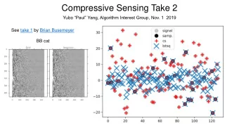
CS Fundamental Missing Data Recovery Theory Challenges Algorithms FPC Total Variation Application: Missing Data Recovery Complete data 0.5 0 −0.5 0 100 200 300 400 500 600 700 800 900 1000 Available data 0.5 0 −0.5 0 100 200 300 400 500 600 700 800 900 1000 Recovered data 0.5 0 −0.5 0 100 200 300 400 500 600 700 800 900 1000 The signal was synthesized by a few Fourier components.

CS Fundamental Missing Data Recovery Theory Challenges Algorithms FPC Total Variation Application: Missing Data Recovery II Complete data Available data Recovered data 75% of pixels were blacked out (becoming unknown).

CS Fundamental Missing Data Recovery Theory Challenges Algorithms FPC Total Variation Application: Missing Data Recovery III Complete data Available data Recovered data 85% of pixels were blacked out (becoming unknown).

CS Fundamental Missing Data Recovery Theory Challenges Algorithms FPC Total Variation How are missing data recovered? Data vector f has a missing part u : � b � b ∈ ℜ m , u ∈ ℜ n − m . f := , u Under a basis Φ , f has a representation x ∗ , f = Φ x ∗ , or � A � b � � x ∗ = . B u Under favorable conditions ( x ∗ is sparse and A is “good”), x ∗ = arg min {� x � 1 : Ax = b } , then we recover missing data u = Bx ∗ .

CS Fundamental Missing Data Recovery Theory Challenges Algorithms FPC Total Variation Sufficient Condition for Recovery F = { x : Ax = Ax ∗ } ≡ { x ∗ + v : v ∈ Null ( A ) } Feasibility: S ∗ = { i : x ∗ Z ∗ = { 1 , · · · , n } \ S ∗ Define: i � = 0 } , � x ∗ � 1 + ( � v Z ∗ � 1 − � v S ∗ � 1 ) + � x � 1 = � � x ∗ S ∗ + v S ∗ � 1 − � x ∗ � S ∗ � 1 + � v S ∗ � 1 � x ∗ � 1 , if � v Z ∗ � 1 > � v S ∗ � 1 > x ∗ is the unique min. if � v � 1 > 2 � v S ∗ � 1 , ∀ v ∈ Null ( A ) \ { 0 } . Since � x ∗ � 1 / 2 � v � 2 ≥ � v S ∗ � 1 , it suffices that 0 � v � 1 > 2 � x ∗ � 1 / 2 � v � 2 , ∀ v ∈ Null ( A ) \ { 0 } 0

CS Fundamental Missing Data Recovery Theory Challenges Algorithms FPC Total Variation ℓ 1 -norm vs. Sparsity Sufficient Sparsity for Unique Recovery: � v � 1 � � x ∗ � 0 < 1 � v � 2 , ∀ v ∈ Null ( A ) \ { 0 } 2 By uniqueness, x � = x ∗ , Ax = Ax ∗ ⇒ � x � 0 > � x ∗ � 0 . Hence, x ∗ arg min {� x � 1 : Ax = Ax ∗ } = arg min {� x � 0 : Ax = Ax ∗ } = i.e., minimum ℓ 1 -norm implies maximum sparsity.

CS Fundamental Missing Data Recovery Theory Challenges Algorithms FPC Total Variation In most subspaces, � v � 1 ≫ � v � 2 � v � 2 ≤ √ n . However, � v � 1 ≫ � v � 2 in most In R n , 1 ≤ � v � 1 subspaces (due to concentration of measure). Theorem: (Kashin 77, Garnaev-Gluskin 84) Let A ∈ R m × n be standard iid Gaussian. With probability above 1 − e − c 1 ( n − m ) , √ m � v � 1 c 2 ≥ , ∀ v ∈ Null ( A ) \ { 0 } � v � 2 � log ( n / m ) where c 1 and c 2 are absolute constants. Immediately, for random A and with high probability Cm log ( n / m ) ⇒ x ∗ is recoverable . � x ∗ � 0 <

CS Fundamental Missing Data Recovery Theory Challenges Algorithms FPC Total Variation Signs help Theorem: There exist good measurement matrices A ∈ R m × n so that if x ∗ ≥ 0 and � x ∗ � 0 ≤ ⌊ m / 2 ⌋ , then x ∗ = arg min {� x � 1 : Ax = Ax ∗ , x ≥ 0 } . In particular, (generalized) Vandermonde matrices (including partial DFT matrices) are good. (“ x ∗ ≥ 0” can be replaced by “ sign ( x ∗ ) is known”.)

CS Fundamental Missing Data Recovery Theory Challenges Algorithms FPC Total Variation Discussion Further Results: Better estimates on constants (still uncertain) Some non-random matrices are good too (e.g. partial transforms) Implications of CS: Theoretically, sample size n → O ( k log ( n / k )) Work-load shift: encoder → decoder New paradigm in data acquisition? In practice, compression ratio not dramatic, but — longer battery life for space devises? — shorter scan time for MRI? ...

CS Fundamental Missing Data Recovery Theory Challenges Algorithms FPC Total Variation Related ℓ 1 -minimization Problems min {� x � 1 : Ax = b } (noiseless) min {� x � 1 : � Ax − b � ≤ ǫ } (noisy) min µ � x � 1 + � Ax − b � 2 (unconstrained) ( Φ − 1 may not exist) min µ � Φ x � 1 + � Ax − b � 2 min µ � G ( x ) � 1 + � Ax − b � 2 ( G ( · ) may be nonlinear) min µ � G ( x ) � 1 + ν � Φ x � 1 + � Ax − b � 2 (mixed form) Φ may represent wavelet or curvelet transform � G ( x ) � 1 can represent isotropic TV (total variation) Objectives are not necessarily strictly convex Objectives are non-differentiable

CS Fundamental Missing Data Recovery Theory Challenges Algorithms FPC Total Variation Algorithmic Challenges Large-scale, non-smooth optimization problems with dense data that require low storage and fast algorithms. 1k × 1k, 2D-images give over 10 6 variables. “Good" matrices are dense (random, transforms...). Often (near) real-time processing is required. Matrix factorizations are out of question. Algorithms must be built on Av and A T v .

CS Fundamental Missing Data Recovery Theory Challenges Algorithms FPC Total Variation Algorithm Classes (I) Greedy Algorithms: Marching Pursuits (Mallat-Zhang, 1993) OMP (Gilbert-Tropp, 2005) StOMP (Donoho et al, 2006) Chaining Pursuit (Gilbert et al, 2006) Cormode-Muthukrishnan (2006) HHS Pursuit (Gilbert et al, 2006) Some require special encoding matrices.

CS Fundamental Missing Data Recovery Theory Challenges Algorithms FPC Total Variation Algorithm Classes (II) Introducing extra variables, one can convert compressive sensing problems into smooth linear or 2nd-order cone programs; e.g. min {� x � 1 : Ax = b } ⇒ LP min { e T x + − e T x − : Ax + − Ax − = b , x + , x − ≥ 0 } Smooth Optimization Methods: Projected Gradient: GPSR (Figueiredo-Nowak-Wright, 07) Interior-point algorithm: ℓ 1 -LS (Boyd et al 2007) (pre-conditioned CG for linear systems) ℓ 1 -Magic (Romberg 2006)

CS Fundamental Missing Data Recovery Theory Challenges Algorithms FPC Total Variation Fixed-Point Shrinkage min µ � x � 1 + f ( x ) ⇐ ⇒ x = Shrink ( x − τ ∇ f ( x ) , τµ ) where Shrink ( y , t ) = sign ( y ) ◦ max ( | y | − t , 0 ) Fixed-point iterations: x k + 1 = Shrink ( x k − τ ∇ f ( x k ) , τµ ) directly follows from forward-backward operator splitting (a long history in PDE and optimization since 1950’s) Rediscovered in signal processing by many since 2000’s. Convergence properties analyzed extensively

CS Fundamental Missing Data Recovery Theory Challenges Algorithms FPC Total Variation Forward-Backward Operator Splitting Derivation: min µ � x � 1 + f ( x ) ⇔ 0 ∈ µ∂ � x � 1 + ∇ f ( x ) ⇔ − τ ∇ f ( x ) ∈ τµ∂ � x � 1 ⇔ x − τ ∇ f ( x ) ∈ x + τµ∂ � x � 1 ⇔ ( I + τµ∂ � · � 1 ) x ∋ x − τ ∇ f ( x ) { x } ∋ ( I + τµ∂ � · � 1 ) − 1 ( x − τ ∇ f ( x )) ⇔ ⇔ x = shrink ( x − τ ∇ f ( x ) , τµ ) min µ � x � 1 + f ( x ) ⇐ ⇒ x = Shrink ( x − τ ∇ f ( x ) , τµ )

CS Fundamental Missing Data Recovery Theory Challenges Algorithms FPC Total Variation New Convergence Results The following are obtained by E. Hale, W, Yin and YZ, 2007. Finite Convergence: for k = O ( 1 /τµ ) x k if x ∗ j = 0 , j = 0 sign ( x k j ) = sign ( x ∗ if x ∗ j ) , J � = 0 Rate of convergence depending on “reduced” Hessian: � x k + 1 − x ∗ � ≤ κ ( H ∗ EE ) − 1 lim sup � x k − x ∗ � κ ( H ∗ EE ) + 1 k →∞ EE is the sub-Hessian corresponding to x ∗ � = 0. where H ∗ The bigger µ is, the sparser x ∗ is, the faster is the convergence.