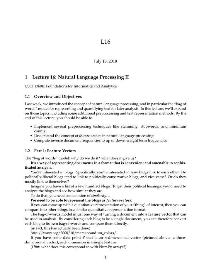

L16 July 18, 2018 1 Lecture 16: Natural Language Processing II CSCI 1360E: Foundations for Informatics and Analytics 1.1 Overview and Objectives Last week, we introduced the concept of natural language processing, and in particular the “bag of words” model for representing and quantifying text for later analysis. In this lecture, we’ll expand on those topics, including some additional preprocessing and text representation methods. By the end of this lecture, you should be able to • Implement several preprocessing techniques like stemming, stopwords, and minimum counts • Understand the concept of feature vectors in natural language processing • Compute inverse document frequencies to up or down-weight term frequencies 1.2 Part 1: Feature Vectors The “bag of words” model: why do we do it? what does it give us? It’s a way of representing documents in a format that is convenient and amenable to sophis- ticated analysis. You’re interested in blogs. Specifically, you’re interested in how blogs link to each other. Do politically-liberal blogs tend to link to politically-conservative blogs, and vice versa? Or do they mostly link to themselves? Imagine you have a list of a few hundred blogs. To get their political leanings, you’d need to analyze the blogs and see how similar they are. To do that, you need some notion of similarity . . . We need to be able to represent the blogs as feature vectors . If you can come up with a quantitative representation of your “thing” of interest, then you can compare it to other things in a similar quantitative representation format. The bag-of-words model is just one way of turning a document into a feature vector that can be used in analysis. By considering each blog to be a single document, you can therefore convert each blog to its own bag-of-words and compare them directly. (in fact, this has actually been done) http://waxy.org/2008/10/memeorandum_colors/ If you have some data point � x that is an n -dimensional vector (pictured above: a three- dimensional vector), each dimension is a single feature. ( Hint : what does this correspond to with NumPy arrays?) 1
blogs featurevector 2
wordvector Therefore, a bag-of-words model is just a way of representing a document as a vector , where each dimension is the count of one specific word! Yes–a single dimension per word. That means, for a document with hundreds of thousands of unique words, the document’s corresponding feature vector (courtesy of the bag-of-words repre- sentation) has hundreds of thousands of dimensions. Pictured above are three separate documents, and the number of times each of the words ap- pears is given by the height of the histogram bar. Stare at this until you get some understanding of what’s happening– these are three documents that share the same words (as you can see, they have the same x-axes), but what differs are the relative heights of the bars , meaning they have differ- ent values along the x-axes. Of course there are other ways of representing documents as vectors, but bag-of-words is the easiest . 1.3 Part 2: Text Preprocessing What is “preprocessing”? Name some preprocessing techniques with text we’ve covered! • Lower case (or upper case) everything • Split into single words • Remove trailing whitespace (spaces, tabs, newlines) There are a few more that can be very powerful. To start, let’s go back to the Alice in Wonderland example from the previous lecture, but this time, we’ll add a few more books for comparison: 3
• Pride and Prejudice , by Jane Austen • Frankenstein , by Mary Shelley • Beowulf , by Lesslie Hall • The Adventures of Sherlock Holmes , by Sir Arthur Conan Doyle • The Adventures of Tom Sawyer , by Mark Twain • The Adventures of Huckleberry Finn , by Mark Twain Hopefully this variety should give us a good idea what we’re dealing with! First, we’ll read all the books’ raw contents into a dictionary. In [1]: books = {} # We'll use a dictionary to store all the text from the books. files = ['Lecture16/alice.txt', 'Lecture16/pride.txt', 'Lecture16/frank.txt', 'Lecture16/bwulf.txt', 'Lecture16/holmes.txt', 'Lecture16/tom.txt', 'Lecture16/finn.txt'] for f in files: # This weird line just takes the part of the filename between the "/" and "." as the prefix = f.split("/")[-1].split(".")[0] try: with open(f, "r", encoding = "ISO-8859-1") as descriptor: books[prefix] = descriptor.read() except: print("File '{}' had an error!".format(f)) books[prefix] = None In [2]: # Here you can see the dict keys (i.e. the results of the weird line of code in the last print(books.keys()) dict_keys(['alice', 'pride', 'frank', 'bwulf', 'holmes', 'tom', 'finn']) Just like before, let’s go ahead and lower case everything, strip out whitespace, then count all the words. In [3]: def preprocess(book): # First, lowercase everything. lower = book.lower() # Second, split into lines. lines = lower.split("\n") # Third, split each line into words. words = [] for line in lines: words.extend(line.strip().split(" ")) 4
# That's it! return count(words) In [4]: from collections import defaultdict # Our good friend from the last lecture, defaultdict! def count(words): # This function takes a list of words as input, and counts them all up. counts = defaultdict(int) for w in words: counts[w] += 1 return counts In [5]: # Finally, let's loop through our books and count # all the words that show up! counts = {} for k, v in books.items(): counts[k] = preprocess(v) Let’s see how our basic preprocessing techniques from the last lecture worked out. In [6]: from collections import Counter def print_results(counts): for key, bag_of_words in counts.items(): word_counts = Counter(bag_of_words) # Remember "Counter"? mc_word, mc_count = word_counts.most_common(1)[0] print("'{}': {} unique words; most common word '{}' appeared {} times." .format(key, len(bag_of_words.keys()), mc_word, mc_count)) print_results(counts) 'alice': 5582 unique words; most common word 'the' appeared 1777 times. 'pride': 13128 unique words; most common word 'the' appeared 4479 times. 'frank': 11702 unique words; most common word 'the' appeared 4327 times. 'bwulf': 11024 unique words; most common word '' appeared 3497 times. 'holmes': 14544 unique words; most common word 'the' appeared 5704 times. 'tom': 13445 unique words; most common word 'the' appeared 3907 times. 'finn': 13839 unique words; most common word 'and' appeared 6109 times. Yeesh. Not only are the most common words among the most boring (“the”? “and”?), but there are occasions where the most common word isn’t even a word, but rather a blank space. (How do you think that could happen?) Let’s take a quick step back and think about the code we just saw. • The preprocess function takes a single book string as input and does some preprocessing: it lowercases everything so it’s all the same case, it splits up the string into single words, and it adds all these words to one big list. 5
• We also have a count function, which takes a list of words (output from preprocess ) and counts everything up into a dictionary (the keys are unique words, the values how many times those words appear in the book). • Finally, we have a block of code that loops over all our books and runs these two functions on each of them, building dictionaries of word counts. These are fed into print_results so that we can see 1) the number of unique words in each book, and 2) the most common word in each book. We’re going to repeat this process for the rest of the lecture, slowly upgrading the preprocess function so that the final result (top words for each book) become more meaningful and indicative of the books’ contents. If you had trouble following, please go back over the code again with these points in mind. 1.3.1 Stop words A great first step is to implement stop words. (I used this list of 319 stop words) In [7]: # This code just reads in the words from a stoplist file # and adds them to a list we can use later. with open("Lecture16/stopwords.txt", "r") as f: lines = f.read().split("\n") stopwords = [w.strip() for w in lines] print(stopwords[:5]) ['a', 'about', 'above', 'across', 'after'] We’ll now use the words in the stopwords list to eliminate words from our books (remember: we consider “stop words” to be meaningless to the overall semantics of the text; go back to the previous lecture if you need a refresher on stop words). Now we’ll augment our preprocess function to include stop word processing. In [8]: def preprocess_v2(book, stopwords): # Note the "_v2"--this is a new function! # First, lowercase everything. lower = book.lower() # Second, split into lines. lines = lower.split("\n") # Third, split each line into words. words = [] for line in lines: tokens = line.strip().split(" ") ### NEW CODE HERE! # Check for stopwords. for t in tokens: if t in stopwords: continue # This "continue" SKIPS the stopword entirely! 6
Recommend
More recommend