L ECTURE 9: E VALUATION Prof. Julia Hockenmaier - PowerPoint PPT Presentation
CS446 Introduction to Machine Learning (Fall 2015) University of Illinois at Urbana-Champaign http://courses.engr.illinois.edu/cs446 L ECTURE 9: E VALUATION Prof. Julia Hockenmaier juliahmr@illinois.edu Admin Homework 1 is being graded.
CS446 Introduction to Machine Learning (Fall 2015) University of Illinois at Urbana-Champaign http://courses.engr.illinois.edu/cs446 L ECTURE 9: E VALUATION Prof. Julia Hockenmaier juliahmr@illinois.edu
Admin Homework 1 is being graded. Homework 2: Do not buy Matlab!! We have clarified Problem 1 We have added a readme file for the Matlab part. Project proposals: Submit on Compass by Thursday. CS446 Machine Learning 2
Recap: duals and kernels CS446 Machine Learning 3
Dual representation Classifying x in the primal: f( x ) = w x w = feature weights (to be learned) wx = dot product between w and x Classifying x in the dual: f( x ) = ∑ n α n y n x n x α n = weight of n -th training example (to be learned) x n x = dot product between x n and x The dual representation is advantageous when #training examples ≪ #features (requires fewer parameters to learn) CS446 Machine Learning 4
The kernel trick – Define a feature function φ ( x ) which maps items x into a higher-dimensional space. – The kernel function K( x i , x j ) computes the inner product between the φ ( x i ) and φ ( x j ) K( x i , x j ) = φ ( x i ) φ ( x j ) – Dual representation: We don’t need to learn w in this higher-dimensional space. It is sufficient to evaluate K( x i , x j ) CS446 Machine Learning 5
Constructing kernels We have looked at a few examples of basic kernel functions (e.g. quadratic/polynomial kernels) We have looked at ways to construct more complex kernel functions. CS446 Machine Learning 6
Kernels over (finite) sets X, Z: subsets of a finite set D with |D| elements k (X, Z) = |X ∩ Z| (the number of elements in X and Z) is a valid kernel: k (X, Z) = φ (X) φ (Z) where φ (X) maps X to a bit vector of length |D| ( i- th bit: does X contains the i- th element of D?). k (X, Z) = 2 |X ∩ Z| (the number of subsets shared by X and Z) is a valid kernel: φ (X) maps X to a bit vector of length 2 |D| ( i- th bit: does X contains the i- th subset of D?) CS446 Machine Learning 7
Statistical hypothesis testing CS446 Machine Learning 8
Why hypothesis testing? Q: If Accuracy(A) > Accuracy(B), can we conclude that classifier A is better than B? A: No, not necessarily. Only if the difference between Accuracy(A) and Accuracy(B) is unlikely to arise by chance . CS446 Machine Learning 9
Hypothesis testing We have a hypothesis H that we wish to show is true. (H = “There is a difference between A and B”) We have a statistic M that measures the difference between A and B, and we have measured a value m of M in our data. But m itself doesn’t tell us whether H is true or false. Instead, we estimate how likely m were to arise if the opposite of H (= the ‘null hypothesis’, H 0 ) was true. (H 0 = “There is no difference between A and B”). If P(M ≥ m | H 0 ) < p , we can reject H 0 with p-value p CS446 Machine Learning 10
Rejecting H 0 – H 0 defines a distribution P( M | H 0 ) over some statistic M (e.g. M = the difference in accuracy between A and B) – Select a significance value S (e.g. 0.05, 0.01, etc.) You can only reject H 0 if P(M= m | H 0 ) ≤ S – Compute the test statistic m from your data e.g. the average difference in accuracy over N folds – Compute P( M ≥ m | H 0 ) – Reject H 0 with p -value p ≤ S if P(M ≥ m | H 0 ) ≤ S Caveat: the p -value corresponds to P( m | H 0 ), not P(H 0 | m ) CS446 Machine Learning 11
p -Values Commonly used p -values are: – 0.05: There is a 5% (1/20) chance to get the observed results under the null hypothesis. Corollary: If you run 20 or more experiments, at least one of them will yield results that fall in the “statistically significant range” with p=0.05, even if the null hypothesis is actually true. – 0.01: There is a 1% (1/100) chance to get the observed results under the null hypothesis. CS446 Machine Learning 12
Null hypothesis Null hypothesis: We assume the data comes from a (normal) distribution P( M | H 0 ) with mean µ=0 and (unknown) variance σ 2 / N. 0.5 -2.5 0 2.5 m 1 m 2 From the data (sample) X = {x 1 …x N }, we compute the sample mean m = ∑ i x i / N How likely is it that m came from P( M| H 0 )? For m 1 : very likely. For m 2 : pretty unlikely CS446 Machine Learning 13
Confidence intervals One-tailed test: Test whether the accuracy of A is higher than B with probability p Two-tailed test: Test whether the accuracies of A and B are different (lower or higher) with probability p This is the stricter test. CS446 Machine Learning 14
Confidence intervals One-tailed test: We fail to reject H 0 if m is inside the asymmetric 100(1-p) percent confidence interval (- ∞ , a) Two-tailed test: We fail to reject H 0 if m lies in the symmetric 100(1-p) percent confidence interval (-a, +a) around the mean. p=0.05%; Confidence 95% p=0.05%; Confidence 95% Two-tailed test One-tailed test 0.5 0.5 -2.5 0 2.5 -2.5 0 2.5 Reject H 0 Accept H 0 Reject H 0 Accept H 0 Reject H 0 CS446 Machine Learning 15
Hypothesis tests to evaluate classifiers Paired t-test: Compare the performance of two classifiers on N test sets (e.g. N-fold cross-validation). Uses the t-statistic to compute confidence intervals. McNemar’s test: Compare the performance of two classifiers on N items from a single test set. CS446 Machine Learning 16
N-fold cross validation: Paired t-test CS446 Machine Learning 17
N-fold cross validation Instead of a single test-training split: train � test � – Split data into N equal-sized parts – Train and test N different instances of the same classifier – This gives N different accuracies CS446 Machine Learning 18
Evaluating N-fold cross validation test set 1 test set 2 test set 3 test set 4 test set 5 A 80% 82% 85% 78% 85% B 81% 81% 86% 80% 88% diff (A − B) -1% +1% -1% -2% -3% The paired t-test tells us whether there is a (statistically significant) difference between the accuracies of classifiers A and B, based on their difference in accuracy on N different test sets. CS446 Machine Learning 19
Paired t-test for cross-validation Two different classifiers, A and B are trained and tested using N-fold cross-validation For the n- th fold: accuracy (A, n ), accuracy (B, n ) diff n = accuracy (A, n ) − accuracy (B, n ) Null hypothesis: diff comes from a distribution with mean (expected value) = 0. CS446 Machine Learning 20
Paired t-test Null hypothesis (H 0 ; to be rejected), informally: There is no difference between A and B’s accuracy. – Statistically, we treat accuracy(A) and accuracy(B) as random variables drawn from some distribution. – H 0 says that accuracy(A) and accuracy(B) are drawn from the same distribution. – If H 0 is true, then the expected difference (over all possible data sets) between their accuracies is 0. Null hypothesis (H 0 ; to be rejected), formally: The difference between accuracy(A) and accuracy(B) on the same test set is a random variable with mean = 0. H 0 : E [accuracy(A) – accuracy(B)] = E [ diff D ] = 0 CS446 Machine Learning 21
Paired t-test Null hypothesis (H 0 ; to be rejected), formally: The difference between accuracy(A) and accuracy(B) on the same test set is a random variable with mean = 0. H 0 : E [accuracy(A) – accuracy(B)] = E [ diff D ] = 0 – E [ diff D ] is the expected value (mean) over all possible data sets. We don’t (can’t) know that quantity. – But N- fold cross-validation gives us N samples of diff D We can ask instead: How likely are these N samples to come from a distribution with mean = 0? CS446 Machine Learning 22
Paired t-test Paired t-test: The accuracy of A on test set i is paired with the accuracy of B on test set i Assumption: Accuracies are drawn from a normal distribution (with unknown variance) Null hypothesis: The accuracies of A and B are drawn from the same distribution. Hence, the difference of the accuracies on test set i comes from a normal distribution with mean = 0 Alternative hypothesis: The accuracies are drawn from two different distributions: E[ diff ] ≠ 0 CS446 Machine Learning 23
Paired t-test Given: a sample of N observations We assume these come from a normal distribution with fixed (but unknown) mean and variance – Compute the sample mean and sample variance for these observations – This allows you to compute the t-statistic . – The t-distribution for N-1 degrees of freedom can be used to estimate how likely it is that the true mean is in a given range Reject H 0 at significance level p if the t-statistic does not lie in the interval (- t p /2, n-1 , + t p /2, n-1 ). There are tables where you can look this up CS446 Machine Learning 24
Computing the t-statistic Difference in accuracy on the n -th test set: diff n = Accuracy n (A) – Accuracy n (B) Sample mean m of diff D , based on N samples of diff D : N ∑ m = 1 diff n N n = 1 Sample standard deviation S of diff D : N ( diff n − m ) 2 ∑ S = n = 1 N − 1 t-statistic for N samples of diff D : N ⋅ m t = S CS446 Machine Learning 25
Can we reject H 0 ? 1. Compute the t-statistic t for your N samples. 2. Define a p-value p ∈ {0.05, 0.01, 0.001}. 3. Look up t p/2,N − 1 for N − 1 degrees of freedom (df) 4. If t > t N-1,p : Reject H 0 with p-value p CS446 Machine Learning 26
Recommend
More recommend
Explore More Topics
Stay informed with curated content and fresh updates.
