Krylov methods for tensors I Lars Eldn and Berkant Savas Department - PowerPoint PPT Presentation
Krylov methods for tensors I Lars Eldn and Berkant Savas Department of Mathematics Linkping University, Sweden NSF Workshop, February 2009 Lars Eldn and Berkant Savas (LiU) Tensor-Krylov Methods NSF Workshop, February 2009 1 / 38
Krylov methods for tensors I Lars Eldén and Berkant Savas Department of Mathematics Linköping University, Sweden NSF Workshop, February 2009 Lars Eldén and Berkant Savas (LiU) Tensor-Krylov Methods NSF Workshop, February 2009 1 / 38
Outline Introduction 1 Tensor concepts 2 Matrix-tensor multiplication Inner Product and Norm Contractions Best Approximation 3 Grassmann Optimization Numerical Examples Sparse Tensors: Krylov Methods 4 Conclusions 5 Lars Eldén and Berkant Savas (LiU) Tensor-Krylov Methods NSF Workshop, February 2009 2 / 38
Tech Report Download the tech report from http://www.mai.liu.se/~besav/files/tensorKrylov.pdf Lars Eldén and Berkant Savas (LiU) Tensor-Krylov Methods NSF Workshop, February 2009 3 / 38
Tensor Decomposition: Tucker Model � � U ( 3 ) � � � � � � � � � � = U ( 1 ) U ( 2 ) A S � � � � Tucker 1964, numerous papers in psychometrics and chemometrics De Lathauwer et al., SIMAX 2000: notation, theory. The matrices U ( i ) are usually orthogonal. This talk: Tucker model for 3-tensors only! Generalization straightforward. Lars Eldén and Berkant Savas (LiU) Tensor-Krylov Methods NSF Workshop, February 2009 4 / 38
Mode − I Multiplication of a Tensor by a Matrix Assume that dimensions are such that all operations are well-defined. Mostly 3-tensors. Lim’s notation. (No standard notation yet) n � B = ( X ) 1 · A , B ( i , j , k ) = x i ν a ν jk . ν = 1 All column vectors are multiplied by the matrix X . Multiplication in all modes at the same time: � B = ( X , Y , Z ) · A , B ( i , j , k ) = x i ν y j µ z k λ a νµλ . ν,µ,λ For convenience we write B = ( X T , Y T , Z T ) · A = A · ( X , Y , Z ) Lars Eldén and Berkant Savas (LiU) Tensor-Krylov Methods NSF Workshop, February 2009 5 / 38
Inner Product and Norm Inner product (contraction: R n × n × n → R ) � �A , B� = a ijk b ijk i , j , k The Frobenius norm: �A� = �A , A� 1 / 2 Matrix case � A , B � = tr ( A T B ) Lars Eldén and Berkant Savas (LiU) Tensor-Krylov Methods NSF Workshop, February 2009 6 / 38
Partial Contractions � C = �A , B� 1 , c jklm = a λ jk b λ lm , (4-tensor) , λ � D = �A , B� 1 : 2 , d jk = a λµ j b λµ k , (2-tensor) , λ,µ � e = �A , B� = �A , B� 1 : 3 , e = a λµν b λµν , (scalar) . λ,µ,ν Notation (3-tensor): �A , B� 1 : 2 = �A , B� − 3 Lars Eldén and Berkant Savas (LiU) Tensor-Krylov Methods NSF Workshop, February 2009 7 / 38
Best Rank − ( r 1 , r 2 , r 3 ) Approximation Z T S Y T ≈ A X Best rank − ( r 1 , r 2 , r 3 ) approximation: X T X = I , Y T Y = I , Z T Z = I X , Y , Z , S �A − ( X , Y , Z ) · S� , min The problem is over-parameterized! Lars Eldén and Berkant Savas (LiU) Tensor-Krylov Methods NSF Workshop, February 2009 8 / 38
Best Approximation rank ( B )=( r 1 , r 2 , r 3 ) �A − B� min is equivalent to X , Y , Z Φ( X , Y , Z ) = 1 2 �A · ( X , Y , Z ) � 2 max 2 = 1 � � , a λµν x λ j y µ k z ν l 2 j , k , l λ,µ,ν subject to X T X = I r 1 , Y T Y = I r 2 , Z T Z = I r 3 Lars Eldén and Berkant Savas (LiU) Tensor-Krylov Methods NSF Workshop, February 2009 9 / 38
Grassmann Optimization The Frobenius norm is invariant under orthogonal transformations: Φ( X , Y , Z ) = Φ( XU , YV , ZW ) = 1 2 �A · ( XU , YV , ZW ) � 2 for orthogonal U ∈ R r 1 × r 1 , V ∈ R r 2 × r 2 , and W ∈ R r 3 × r 3 . Maximize Φ over equivalence classes [ X ] = { XU | U orthogonal } . Product of manifolds: Gr 3 = Gr ( J , r 1 ) × Gr ( K , r 2 ) × Gr ( L , r 3 ) 1 ( X , Y , Z ) ∈ Gr 3 Φ( X , Y , Z ) = max max 2 �A · ( X , Y , Z ) , A · ( X , Y , Z ) � ( X , Y , Z ) ∈ Gr 3 Lars Eldén and Berkant Savas (LiU) Tensor-Krylov Methods NSF Workshop, February 2009 10 / 38
Methods for Best Approximation Grassmann-based Newton (LE, B. Savas) 1 Trust region/Newton (Ishteva, De Lathauwer et al.) 2 BFGS quasi-Newton (Savas, Lim) 3 Limited memory BFGS (Savas, Lim) 4 Alternating HOOI (Kroonenberg, De Lathauwer) 1 Lars Eldén and Berkant Savas (LiU) Tensor-Krylov Methods NSF Workshop, February 2009 11 / 38
Numerical Example I BFGS L−BFGS HOOI RELATIVE NORM OF THE GRADIENT NG −5 10 −10 10 −15 10 0 20 40 60 80 100 ITERATION # A random tensor A ∈ R 20 × 20 × 20 with random entries N(0, 1) approximated with a rank − ( 5 , 5 , 5 ) tensor. Lars Eldén and Berkant Savas (LiU) Tensor-Krylov Methods NSF Workshop, February 2009 12 / 38
Numerical Example II BFGS L−BFGS HOOI RELATIVE NORM OF THE GRADIENT −5 10 −10 10 −15 10 200 300 400 500 600 700 800 ITERATION # A random tensor A ∈ R 100 × 100 × 100 with random entries N(0, 1) approximated with a rank − ( 5 , 10 , 20 ) tensor. Lars Eldén and Berkant Savas (LiU) Tensor-Krylov Methods NSF Workshop, February 2009 13 / 38
Sparse Tensors in Information Sciences In information sciences the tensors are often sparse: Term-document-author analysis (Dunlavy et al) Graphs, web link analysis (Kolda et al, PARAFAC model) � 1 if page i points to page j using term k a ijk = 0 otherwise Lars Eldén and Berkant Savas (LiU) Tensor-Krylov Methods NSF Workshop, February 2009 14 / 38
Web page with links Lars Eldén and Berkant Savas (LiU) Tensor-Krylov Methods NSF Workshop, February 2009 15 / 38
Sparse Matrices Krylov methods give low rank approximations: AV k = U k H k = U k H k V T k . ≈ A The matrix is only used as operator: u = Av Lars Eldén and Berkant Savas (LiU) Tensor-Krylov Methods NSF Workshop, February 2009 16 / 38
Sparse Tensors Can we generalize Krylov methods to tensors and obtain low rank approximations? Z T S Y T ≈ A X Lars Eldén and Berkant Savas (LiU) Tensor-Krylov Methods NSF Workshop, February 2009 17 / 38
Golub-Kahan Bidiagonalization for Rectangular Matrix β 1 u 1 = b , v 0 = 0 for i = 1 : k α i v i = A T u i − β i v i − 1 , β i + 1 u i + 1 = Av i − α i u i end The coefficients α i and β i are chosen to normalize the vectors. Lars Eldén and Berkant Savas (LiU) Tensor-Krylov Methods NSF Workshop, February 2009 18 / 38
Golub-Kahan Bidiagonalization for Rectangular Matrix β 1 u 1 = b , v 0 = 0 for i = 1 : k α i v i = A T u i − β i v i − 1 , [ α i v i = A · ( u i ) 1 − β i v i − 1 , ] β i + 1 u i + 1 = Av i − α i u i [ β i + 1 u i + 1 = A · ( v i ) 2 − α i u i ] end The coefficients α i and β i are chosen to normalize the vectors. Lars Eldén and Berkant Savas (LiU) Tensor-Krylov Methods NSF Workshop, February 2009 19 / 38
Krylov Method for Tensor Approximation Arnoldi style (i.e., including Gram-Schmidt orthogonalization) Let u 1 and v 1 be given h 111 w 1 = A · ( u 1 , v 1 ) 1 , 2 for ν = 2 : m h u = A · ( U ν − 1 , v ν − 1 , w ν − 1 ) h ν,ν − 1 ,ν − 1 u ν = A · ( v ν − 1 , w ν − 1 ) 2 , 3 − U ν − 1 h u h v = A · ( u ν , V ν − 1 , w ν − 1 ) h ν,ν,ν − 1 v ν = A · ( u ν , w ν − 1 ) 1 , 3 − V ν − 1 h v h w = A · ( u ν , v ν , W ν − 1 ) h ννν w ν = A · ( u ν , v ν ) 1 , 2 − W ν − 1 h w end Approximate � � U T m , V T m , W T A ≈ ( U m , V m , W m ) · H , H = · A m Lars Eldén and Berkant Savas (LiU) Tensor-Krylov Methods NSF Workshop, February 2009 20 / 38
Krylov Method Arnoldi style (i.e., including Gram-Schmidt orthogonalization) Let u 1 and v 1 be given h 111 w 1 = A · ( u 1 , v 1 ) 1 , 2 for ν = 2 : m h u = A · ( U ν − 1 , v ν − 1 , w ν − 1 ) h ν,ν − 1 ,ν − 1 u ν = A · ( v ν − 1 , w ν − 1 ) 2 , 3 − U ν − 1 h u h v = A · ( u ν , V ν − 1 , w ν − 1 ) h ν,ν,ν − 1 v ν = A · ( u ν , w ν − 1 ) 1 , 3 − V ν − 1 h v h w = A · ( u ν , v ν , W ν − 1 ) h ννν w ν = A · ( u ν , v ν ) 1 , 2 − W ν − 1 h w end Lars Eldén and Berkant Savas (LiU) Tensor-Krylov Methods NSF Workshop, February 2009 21 / 38
Gram-Schmidt, closer look for ν = 2 : m h u = A · ( U ν − 1 , v ν − 1 , w ν − 1 ) h ν,ν − 1 ,ν − 1 u ν = A · ( v ν − 1 , w ν − 1 ) 2 , 3 − U ν − 1 h u . . . . . . end The algebra is straightforward: h u is a vector u -vectors live in first mode, U ν − 1 = ( u 1 , u 2 , . . . , u ν − 1 ) Multiply by U ν − 1 in first mode: h ν,ν − 1 ,ν − 1 U T ν − 1 u ν = A · ( U ν − 1 , v ν − 1 , w ν − 1 ) − h u = 0 Lars Eldén and Berkant Savas (LiU) Tensor-Krylov Methods NSF Workshop, February 2009 22 / 38
Minimal Krylov Method Let u 1 and v 1 be given h 111 w 1 = A · ( u 1 , v 1 ) 1 , 2 for ν = 2 : m h u = A · ( U ν − 1 , v ν − 1 , w ν − 1 ) h ν,ν − 1 ,ν − 1 u ν = A · ( v ν − 1 , w ν − 1 ) 2 , 3 − U ν − 1 h u h v = A · ( u ν , V ν − 1 , w ν − 1 ) h ν,ν,ν − 1 v ν = A · ( u ν , w ν − 1 ) 1 , 3 − V ν − 1 h v h w = A · ( u ν , v ν , W ν − 1 ) h ννν w ν = A · ( u ν , v ν ) 1 , 2 − W ν − 1 h w end Richer combinatorial structure: Let µ ≤ ν − 1 and λ ≤ ν − 1: h u = A · ( U ν − 1 , v µ , w λ ) hu ν = A · ( v µ , w λ ) 2 , 3 − U ν − 1 h u Lars Eldén and Berkant Savas (LiU) Tensor-Krylov Methods NSF Workshop, February 2009 23 / 38
Recommend
More recommend
Explore More Topics
Stay informed with curated content and fresh updates.
