JUMP DRIVEN PREPAYMENT AND DEFAULT MODELS FOR LCDS, ABS AND - PowerPoint PPT Presentation
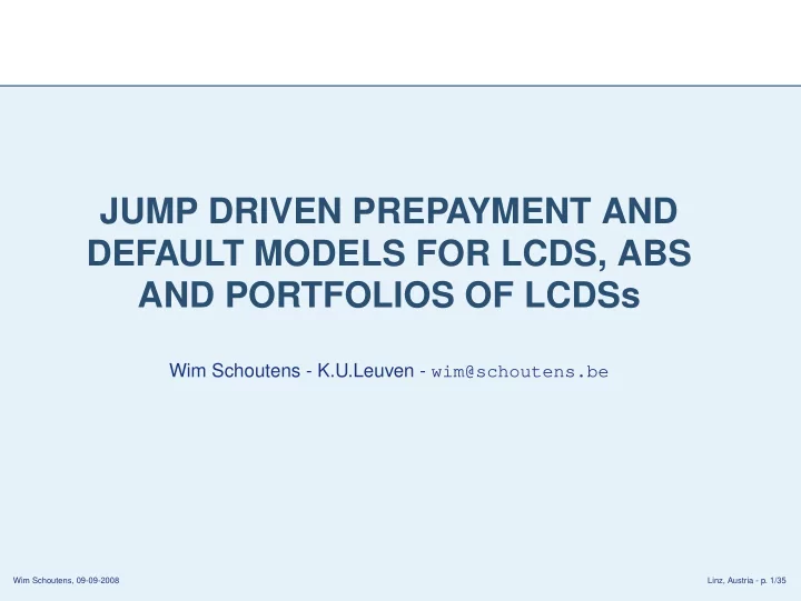
JUMP DRIVEN PREPAYMENT AND DEFAULT MODELS FOR LCDS, ABS AND PORTFOLIOS OF LCDSs Wim Schoutens - K.U.Leuven - wim@schoutens.be Wim Schoutens, 09-09-2008 Linz, Austria - p. 1/35 Joint Work Joao Garcia (Dexia Holding) Serge Goossens (Dexia
JUMP DRIVEN PREPAYMENT AND DEFAULT MODELS FOR LCDS, ABS AND PORTFOLIOS OF LCDSs Wim Schoutens - K.U.Leuven - wim@schoutens.be Wim Schoutens, 09-09-2008 Linz, Austria - p. 1/35
Joint Work ■ Joao Garcia (Dexia Holding) ■ Serge Goossens (Dexia Bank) Outline ■ Hansjörg Albrecher (TU Graz) ● Joint Work ● Content ■ Sophie Ladoucette (Secura Re) Introduction ■ Victoriya Masol (EURANDOM) ABS Modeling ■ Peter Dobranszky (K.U.Leuven - Finalyse) LCDX Modeling Conclusion ■ Geert Van Damme (K.U.Leuven) ■ Marcella Belluci (EIB) Wim Schoutens, 09-09-2008 Linz, Austria - p. 2/35
Content ■ Introduction ◆ Basic of jump processes Outline ■ ABS Modeling ● Joint Work ● Content ◆ Default Fraction Models Introduction ◆ Prepayment Fraction Models ABS Modeling ◆ Impact on Rating and WAL LCDX Modeling ■ LCDX Modeling Conclusion ◆ LCDS implied default and prepayment ◆ Joint modeling of prepayment and default ◆ LCDX one factor model ◆ LCDX base correlation Wim Schoutens, 09-09-2008 Linz, Austria - p. 3/35
Why Lévy ? ■ Credit market events are very shock driven. ■ Jumps and heavy tails are important features in the modeling. Outline Introduction Gamma tail (a=3, b=2) versus Gaussian tail with same mean and variance 0.25 ● Why Lévy ? Gamma tail ● What is a Lévy process ? Gaussian tail ● Defining a Lévy process ● Examples of Lévy : Gamma 0.2 ABS Modeling LCDX Modeling 0.15 Conclusion f(x) 0.1 0.05 0 2.5 3 3.5 4 4.5 5 x Wim Schoutens, 09-09-2008 Linz, Austria - p. 4/35
What is a Lévy process ? ■ Lévy processes are generalization of Brownian Motions (stationary and independent increments) allowing for ◆ non-Gaussian underlying distribution (skewness, kurtosis, more heavier Outline Introduction tails, ...); ● Why Lévy ? ◆ jumps. ● What is a Lévy process ? ● Defining a Lévy process ● Examples of Lévy : Gamma Standard Brownian Motion VG Process (C=20; G=40; M=50) 1 0.1 ABS Modeling 0.8 LCDX Modeling 0.05 0.6 Conclusion 0.4 0 0.2 0 −0.05 −0.2 −0.4 −0.1 −0.6 −0.8 −0.15 0 0.1 0.2 0.3 0.4 0.5 0.6 0.7 0.8 0.9 1 0 0.1 0.2 0.3 0.4 0.5 0.6 0.7 0.8 0.9 1 Wim Schoutens, 09-09-2008 Linz, Austria - p. 5/35
Defining a Lévy process ■ Formal definition: X = { X t , t ≥ 0 } is a Lévy process if ◆ X 0 = 0 ◆ X has independent increments Outline ◆ X has stationary increments Introduction ● Why Lévy ? ◆ the increment X t + s − X t follows a infinitely divisible distribution. ● What is a Lévy process ? ● Defining a Lévy process ■ Examples of infinitely divisible distributions: ● Examples of Lévy : Gamma ◆ Normal → Brownian motion ABS Modeling ◆ Poisson → Poisson process LCDX Modeling ◆ Gamma → Gamma process Conclusion ◆ IG → IG process ◆ CMY → CMY process ◆ Variance Gamma → VG process ◆ Normal Inverse Gaussian → NIG process ◆ Meixner → Meixner process ◆ Generalized Hyperbolic → GH process ◆ etc. Wim Schoutens, 09-09-2008 Linz, Austria - p. 6/35
Examples of Lévy : Gamma ■ The density function of the Gamma distribution Gamma ( a, b ) with parameters a > 0 and b > 0 is given by: Outline b a Γ( a ) x a − 1 exp( − xb ) , Introduction f Gamma ( x ; a, b ) = x > 0 . ● Why Lévy ? ● What is a Lévy process ? ● Defining a Lévy process ■ The Gamma-process G = { G t , t ≥ 0 } with parameters a, b > 0 is a ● Examples of Lévy : Gamma stochastic process which starts at zero and has stationary, independent ABS Modeling Gamma-distributed increments and G t follows a Gamma ( at, b ) distribution. LCDX Modeling Conclusion Gamma Process − ν = 0.15 1.4 1.2 1 0.8 0.6 0.4 0.2 0 0 0.2 0.4 0.6 0.8 1 Wim Schoutens, 09-09-2008 Linz, Austria - p. 7/35
Model Overview ■ We model the default and prepayment fraction of ABS of a certain class of loans which can prepay and default. Outline ■ Default Models: Introduction ◆ logistic ABS Modeling ◆ Cox (Gamma) ● Model Overview ● Logistic Default Model ◆ one-factor (Gaussian and Lévy) ● Cox Default Models ● Cox Gamma Default Model ■ Prepayment Models: ● Gaussian Copula Model ● Tails ◆ Constant Prepayment Rate ● Correlation via Running Time ◆ Cox (Gamma) ● Idea works for every Lévy Processes ● Lévy Copula Model ◆ one-factor (Gaussian and Lévy) ● Gaussian Copula Model : Example ● Constant Prepayment Rate ● Constant Prepayment Rate ● Cox prepayment Model ● 1-factor prepayment models ● ABS Modeling ● ABS Modeling Example LCDX Modeling Conclusion Wim Schoutens, 09-09-2008 Linz, Austria - p. 8/35
Logistic Default Model ■ The Logistic curve a F ( t ) = 1 + b e − c ( t − t 0 ) , Outline ■ a has to be chosen from a predetermined default distribution, e.g. the Introduction Log-Normal distribution with mean µ and standard deviation σ . ABS Modeling ● Model Overview ■ Each different value for a will give rise to a new default curve. ● Logistic Default Model ● Cox Default Models ● Cox Gamma Default Model Logistic default curves ( µ = 0.20 , σ = 0.10) Probability density of LogN( µ = 0.20 , σ = 0.10) ● Gaussian Copula Model ● Tails a = 0.4133 a = 0.3679 ● Correlation via Running Time a = 0.2234 0.5 0.5 a = 0.1047 ● Idea works for every Lévy a = 0.0804 Processes ● Lévy Copula Model 0.4 0.4 X ∼ LogN( µ , σ ) ● Gaussian Copula Model : Example F(t) 0.3 0.3 ● Constant Prepayment Rate ● Constant Prepayment Rate 0.2 0.2 ● Cox prepayment Model ● 1-factor prepayment models 0.1 0.1 ● ABS Modeling ● ABS Modeling Example 0 0 0 20 40 60 80 100 120 0 1 2 3 4 5 6 t f X LCDX Modeling Conclusion Wim Schoutens, 09-09-2008 Linz, Austria - p. 9/35
Cox Default Models ■ Based on a on a single sided Lévy process X = { X t , t ≥ 0 } . ■ The fraction of loans that have defaulted (prepaid) at time t : Outline 1 − exp( − X t ) . Introduction ABS Modeling ■ Hence the fraction of loans that have not defaulted (prepaid) equals ● Model Overview ● Logistic Default Model ● Cox Default Models exp( − X t ) . ● Cox Gamma Default Model ● Gaussian Copula Model ● Tails ■ ∆ t time later the number of loans that by then have not defaulted (prepaid) ● Correlation via Running Time ● Idea works for every Lévy equals exp( − X t +∆ t ) . Processes ● Lévy Copula Model ● Gaussian Copula Model : ■ Hence Example ● Constant Prepayment Rate ● Constant Prepayment Rate (1 − exp( − X t +∆ t )) − (1 − exp( − X t )) ● Cox prepayment Model ● 1-factor prepayment models ● ABS Modeling exp( − X t ) ● ABS Modeling Example LCDX Modeling log(exp( − X t )) − log(exp( − X t +∆ t )) ≈ Conclusion = X t +∆ t − X t . Wim Schoutens, 09-09-2008 Linz, Austria - p. 10/35
Cox Gamma Default Model ■ Based on a Gamma Process G = { G t , t ≥ 0 } : ■ The percentage number of new defaults (prepayments) in each period of Outline length ∆ t is Gamma ( a ∆ t, b ) distributed. Introduction ■ One can match a and b to a preset mean number and variance of defaults ABS Modeling at maturity: ● Model Overview ● Logistic Default Model ● Cox Default Models 1 − (1 + 1 /b ) − aT = µ G ( T ); E [1 − exp( − G T )] = ● Cox Gamma Default Model ● Gaussian Copula Model (1 + 2 /b ) − aT − (1 + 1 /b ) − 2 aT = σ 2 ● Tails V ar [1 − exp( − G T )] = G ( T ) . ● Correlation via Running Time ● Idea works for every Lévy Processes ● Lévy Copula Model Probability density of 1−e − λ (T) , with λ (T) ∼ Gamma(aT = 2.99, b = 12.90) Cox default curve ( µ = 0.20 , σ = 0.10) ● Gaussian Copula Model : Example ● Constant Prepayment Rate 0.5 0.5 ● Constant Prepayment Rate ● Cox prepayment Model 0.4 0.4 ● 1-factor prepayment models X ∼ 1−e − λ (T) ● ABS Modeling P d (t) 0.3 0.3 ● ABS Modeling Example LCDX Modeling 0.2 0.2 Conclusion 0.1 0.1 0 0 0 20 40 60 80 100 120 0 0.5 1 1.5 2 2.5 3 3.5 4 4.5 t f X Wim Schoutens, 09-09-2008 Linz, Austria - p. 11/35
Gaussian Copula Model ■ The Gaussian one-factor model (Vasicek, Li) assumes the following "dynamics" for the standardized firm’s latent value: ◆ A i ( T ) = √ ρ Y + √ 1 − ρ ǫ i , i = 1 , . . . , n ; Outline ◆ where Y and ǫ i , i = 1 , . . . , n are i.i.d. standard normal variables. Introduction ABS Modeling ■ The i th obligor defaults at time T if A i ( T ) falls below some preset barrier ● Model Overview ● Logistic Default Model K i ( T ) (for CDOs extracted from CDS quotes to match individual default ● Cox Default Models ● Cox Gamma Default Model probabilities). ● Gaussian Copula Model ● Tails ■ This model is actual based on the Multivariate Normal / Gaussian Copula ● Correlation via Running Time ● Idea works for every Lévy with its known problems (cfr. correlation smile in CDO models). Processes ● Lévy Copula Model ● Gaussian Copula Model : Example ● Constant Prepayment Rate ● Constant Prepayment Rate ● Cox prepayment Model ● 1-factor prepayment models ● ABS Modeling ● ABS Modeling Example LCDX Modeling Conclusion Wim Schoutens, 09-09-2008 Linz, Austria - p. 12/35
Recommend
More recommend
Explore More Topics
Stay informed with curated content and fresh updates.


