Introduction to Natural Language Processing a course taught as - - PowerPoint PPT Presentation

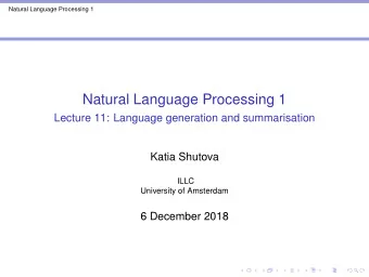
Introduction to Natural Language Processing

a course taught as B4M36NLP at Open Informatics by members of the Institute of Formal and Applied Linguistics Today: Week 1, lecture Today’s topic: Introduction & Probability & Information theory Today’s teacher: Jan Hajiˇ c

E-mail: hajic@ufal.mff.cuni.cz WWW: http://ufal.mff.cuni.cz/jan-hajic

Jan Hajiˇ c (´ UFAL MFF UK) Introduction & Probability & Information theory Week 1, lecture 1 / 1

2016/7

Intro to NLP

• Instructor: Jan Hajič

– ÚFAL MFF UK, office: 420 / 422 MS – Hours: J. Hajic: Mon 9:00-10:00 – preferred contact: hajic@ufal.mff.cuni.cz

• Room & time:

– lecture: Wed, 9:15-10:45 – seminar [cvičení] follows (Zdenek Zabokrtsky) – Oct 5, 2016 – Jan 4, 2017 – Final written exam date: Jan 11, 2017

UFAL MFF UK @ FEL/Intro to Statistical NLP I/Jan Hajic 2

2016/7

Textbooks you need

• Manning, C. D., Schütze, H.:
• Foundations of Statistical Natural Language Processing. The MIT Press.
• 1999. ISBN 0-262-13360-1. [available at least at MFF / Computer

Science School library, Malostranske nam. 25, 11800 Prague 1]

• Jurafsky, D., Martin, J.H.:
• Speech and Language Processing. Prentice-Hall. 2000. ISBN 0-13-095069-6

and newer editions. [recommended].

• Cover, T. M., Thomas, J. A.:

– Elements of Information Theory. Wiley. 1991. ISBN 0-471-06259-6.

• Jelinek, F.:

– Statistical Methods for Speech Recognition. The MIT Press. 1998. ISBN 0-262- 10066-5

UFAL MFF UK @ FEL/Intro to Statistical NLP I/Jan Hajic 3

2016/7

Other reading

• Journals:

– Computational Lingusitics – Transactions on Computational Linguistics

• Proceedings of major conferences:

– ACL (Assoc. of Computational Linguistics) – EACL (European Chapter of ACL) – EMNLP (Empirical Methods in NLP) – CoNLL (Natural Language Learning in CL) – IJCNLP (Asian cahpter of ACL) – COLING (Intl. Committee of Computational Linguistics)

UFAL MFF UK @ FEL/Intro to Statistical NLP I/Jan Hajic 4

2016/7

Course segments (first three lectures)

• Intro & Probability & Information Theory

– The very basics: definitions, formulas, examples.

• Language Modeling

– n-gram models, parameter estimation – smoothing (EM algorithm)

• Hidden Markov Models

– background, algorithms, parameter estimation

UFAL MFF UK @ FEL/Intro to Statistical NLP I/Jan Hajic 5

Probability

2016/7

Experiments & Sample Spaces

• Experiment, process, test, ...
• Set of possible basic outcomes: sample space 

– coin toss ( = {head,tail}), die ( = {1..6}) – yes/no opinion poll, quality test (bad/good) ( = {0,1}) – lottery (|  |  – # of traffic accidents somewhere per year ( = N) – spelling errors ( = *), where Z is an alphabet, and Z* is a set of possible strings over such and alphabet – missing word (|  |  vocabulary size)

UFAL MFF UK @ FEL/Intro to Statistical NLP I/Jan Hajic 7

2016/7

Events

• Event A is a set of basic outcomes
• Usually A and all A 2 (the event space)

–  is then the certain event, is the impossible event

• Example:

– experiment: three times coin toss

•  = {HHH, HHT, HTH, HTT, THH, THT, TTH, TTT}

– count cases with exactly two tails: then

• A = {HTT, THT, TTH}

– all heads:

• A = {HHH}

UFAL MFF UK @ FEL/Intro to Statistical NLP I/Jan Hajic 8

2016/7

Probability

• Repeat experiment many times, record how many

times a given event A occurred (“count” c1).

• Do this whole series many times; remember all cis.
• Observation: if repeated really many times, the

ratios of ci/Ti (where Ti is the number of experiments run in the i-th series) are close to some (unknown but) constant value.

• Call this constant a probability of A. Notation: p(A)

UFAL MFF UK @ FEL/Intro to Statistical NLP I/Jan Hajic 9

2016/7

Estimating probability

• Remember: ... close to an unknown constant.
• We can only estimate it:

– from a single series (typical case, as mostly the outcome of a series is given to us and we cannot repeat the experiment), set p(A) = c1/T1. – otherwise, take the weighted average of all ci/Ti (or, if the data allows, simply look at the set of series as if it is a single long series).

• This is the best estimate.

UFAL MFF UK @ FEL/Intro to Statistical NLP I/Jan Hajic 10

2016/7

Example

• Recall our example:

– experiment: three times coin toss

•  = {HHH, HHT, HTH, HTT, THH, THT, TTH, TTT}

– count cases with exactly two tails: A = {HTT, THT, TTH}

• Run an experiment 1000 times (i.e. 3000 tosses)
• Counted: 386 cases with two tails (HTT, THT, or TTH)
• estimate: p(A) = 386 / 1000 = .386
• Run again: 373, 399, 382, 355, 372, 406, 359

– p(A) = .379 (weighted average) or simply 3032 / 8000

• Uniform distribution assumption: p(A) = 3/8 = .375

UFAL MFF UK @ FEL/Intro to Statistical NLP I/Jan Hajic 11

2016/7

Basic Properties

• Basic properties:

– p: 2 [0,1] – p() = 1 – Disjoint events: p(Ai) = i p(Ai)

• [NB: axiomatic definition of probability: take the

above three conditions as axioms]

• Immediate consequences:

– p() = 0, p(A ) = 1 - p(A), A p(A)  p(B) – a p(a) = 1

UFAL MFF UK @ FEL/Intro to Statistical NLP I/Jan Hajic 12

2016/7

Joint and Conditional Probability

• p(A,B) = p(A B)
• p(A|B) = p(A,B) / p(B)

– Estimating form counts:

• p(A|B) = p(A,B) / p(B) = (c(A  B) / T) / (c(B) / T) =

= c(A  B) / c(B)



A B A  B

UFAL MFF UK @ FEL/Intro to Statistical NLP I/Jan Hajic 13

2016/7

Bayes Rule

• p(A,B) = p(B,A) since p(A p(B 

– therefore: p(A|B) p(B) = p(B|A) p(A), and therefore p(A|B) = p(B|A) p(A) / p(B) ! 

A B A  B

UFAL MFF UK @ FEL/Intro to Statistical NLP I/Jan Hajic 14

2016/7

Independence

• Can we compute p(A,B) from p(A) and p(B)?
• Recall from previous foil:

p(A|B) = p(B|A) p(A) / p(B) p(A|B) p(B) = p(B|A) p(A) p(A,B) = p(B|A) p(A) ... we’re almost there: how p(B|A) relates to p(B)? – p(B|A) = P(B) iff A and B are independent

• Example: two coin tosses, weather today and weather on

March 4th 1789;

• Any two events for which p(B|A) = P(B)!

UFAL MFF UK @ FEL/Intro to Statistical NLP I/Jan Hajic 15

2016/7

Chain Rule

p(A1, A2, A3, A4, ..., An) = !

p(A1|A2,A3,A4,...,An) p(A2|A3,A4,...,An)   p(A3|A4,...,An)  ... p(An-1|An)  p(An)

• this is a direct consequence of the Bayes rule.

UFAL MFF UK @ FEL/Intro to Statistical NLP I/Jan Hajic 16

2016/7

The Golden Rule

(of Classic Statistical NLP)

• Interested in an event A given B (when it is not easy or

practical or desirable to estimate p(A|B)):

• take Bayes rule, max over all As:
• argmaxA p(A|B) = argmaxA p(B|A) . p(A) / p(B) =

argmaxA p(B|A) p(A) !

• ... as p(B) is constant when changing As

UFAL MFF UK @ FEL/Intro to Statistical NLP I/Jan Hajic 17

2016/7

Random Variable

• is a function X: Q

– in general: Q = Rn, typically R – easier to handle real numbers than real-world events

• random variable is discrete if Q is countable (i.e. also if

finite)

• Example: die: natural “numbering” [1,6], coin: {0,1}
• Probability distribution:

– pX(x) = p(X=x) =df p(Ax) where Ax = {a  : X(a) = x} – often just p(x) if it is clear from context what X is

UFAL MFF UK @ FEL/Intro to Statistical NLP I/Jan Hajic 18

2016/7

Expectation Joint and Conditional Distributions

• is a mean of a random variable (weighted average)

– E(X) = xX( x . pX(x)

• Example: one six-sided die: 3.5, two dice (sum) 7
• Joint and Conditional distribution rules:

– analogous to probability of events

• Bayes: pX|Y(x,y) =notation pXY(x|y) =even simpler notation

p(x|y) = p(y|x) . p(x) / p(y)

• Chain rule: p(w,x,y,z) = p(z).p(y|z).p(x|y,z).p(w|x,y,z)

UFAL MFF UK @ FEL/Intro to Statistical NLP I/Jan Hajic 19

Essential Information Theory

2016/7

The Notion of Entropy

• Entropy ~ “chaos”, fuzziness, opposite of order, ...

– you know it:

• it is much easier to create “mess” than to tidy things up...
• Comes from physics:

– Entropy does not go down unless energy is applied

• Measure of uncertainty:

– if low... low uncertainty; the higher the entropy, the higher uncertainty, but the higher “surprise” (information) we can get out of an experiment

UFAL MFF UK @ FEL/Intro to Statistical NLP I/Jan Hajic 21

2016/7

The Formula

• Let pX(x) be a distribution of random variable X
• Basic outcomes (alphabet)

H(X) = -x p(x) log2 p(x) !

• Unit: bits (log10: nats)
• Notation: H(X) = Hp(X) = H(p) = HX(p) = H(pX)

UFAL MFF UK @ FEL/Intro to Statistical NLP I/Jan Hajic 22

2016/7

Using the Formula: Example

• Toss a fair coin:  = {head,tail}

– p(head) = .5, p(tail) = .5 – H(p) = - 0.5 log2(0.5) + (- 0.5 log2(0.5)) = 2  ( (- 0.5)  (-1) ) = 2  0.5 = 1

• Take fair, 32-sided die: p(x) = 1 / 32 for every side x

– H(p) = -i = 1..32 p(xi) log2p(xi) = - 32 (p(x1) log2p(x1) (since for all

i p(xi) = p(x1) = 1/32) = -32  ((1/32)  (- 5)) = 5 (now you see why it’s called bits?)

• Unfair coin:

– p(head) = .2 ... H(p) = .722; p(head) = .01 ... H(p) = .081

UFAL MFF UK @ FEL/Intro to Statistical NLP I/Jan Hajic 23

2016/7

Example: Book Availability

Entropy H(p)

1

bad bookstore

good bookstore

0 0.5 1 p(Book Available)

UFAL MFF UK @ FEL/Intro to Statistical NLP I/Jan Hajic 24

2016/7

The Limits

• When H(p) = 0?

– if a result of an experiment is known ahead of time: – necessarily:

x ; p(x) = 1 & y; y  x  p(y) = 0

• Upper bound?

– none in general – for |  | = n: H(p) log2n

• nothing can be more uncertain than the uniform distribution

UFAL MFF UK @ FEL/Intro to Statistical NLP I/Jan Hajic 25

2016/7

Perplexity: motivation

• Recall:

– 2 equiprobable outcomes: H(p) = 1 bit – 32 equiprobable outcomes: H(p) = 5 bits – 4.3 billion equiprobable outcomes: H(p) ~= 32 bits

• What if the outcomes are not equiprobable?

– 32 outcomes, 2 equiprobable at .5, rest impossible:

• H(p) = 1 bit

– Any measure for comparing the entropy (i.e. uncertainty/difficulty of prediction) (also) for random variables with different number of outcomes?

UFAL MFF UK @ FEL/Intro to Statistical NLP I/Jan Hajic 26

2016/7

Perplexity

• Perplexity:

– G(p) = 2H(p)

• ... so we are back at 32 (for 32 eqp. outcomes), 2 for

fair coins, etc.

• it is easier to imagine:

– NLP example: vocabulary size of a vocabulary with uniform distribution, which is equally hard to predict

• the “wilder” (biased) distribution, the better:

– lower entropy, lower perplexity

UFAL MFF UK @ FEL/Intro to Statistical NLP I/Jan Hajic 27

2016/7

Joint Entropy and Conditional Entropy

• Two random variables: X (space ),Y ()
• Joint entropy:

– no big deal: ((X,Y) considered a single event):

H(X,Y) = -xyp(x,y) log2 p(x,y)

• Conditional entropy:

H(Y|X) = -xyp(x,y) log2 p(y|x) recall that H(X) = E(log2(1/pX(x)))

(weighted average: weights are not conditional)

UFAL MFF UK @ FEL/Intro to Statistical NLP I/Jan Hajic 28

2016/7

Properties of Entropy I

• Entropy is non-negative:

– H(X)  – proof: (recall: H(X) = - x p(x) log2 p(x))

• log(p(x)) is negative or zero for x  1,
• p(x) is non-negative; their product p(x)log(p(x) is thus negative;
• sum of negative numbers is negative;
• and -f is positive for negative f
• Chain rule:

– H(X,Y) = H(Y|X) + H(X), as well as – H(X,Y) = H(X|Y) + H(Y) (since H(Y,X) = H(X,Y))

UFAL MFF UK @ FEL/Intro to Statistical NLP I/Jan Hajic 30

2016/7

Properties of Entropy II

• Conditional Entropy is better (than unconditional):

– H(Y|X)  H(Y)

• H(X,Y)  H(X) + H(Y) (follows from the previous (in)equalities)
• equality iff X,Y independent
• [recall: X,Y independent iff p(X,Y) = p(X)p(Y)]
• H(p) is concave (remember the book availability graph?)

– concave function f over an interval (a,b): x,y (a,b),   [0,1]: f(x + (1-)y) f(x) + (1-)f(y)

• function f is convex if -f is concave

f x y

 f ( x ) + ( 1

• 

) f ( y ) UFAL MFF UK @ FEL/Intro to Statistical NLP I/Jan Hajic 31

2016/7

“Coding” Interpretation of Entropy

• The least (average) number of bits needed to

encode a message (string, sequence, series,...) (each element having being a result of a random process with some distribution p): = H(p)

• Remember various compressing algorithms?

– they do well on data with repeating (= easily predictable = low entropy) patterns – their results though have high entropy  compressing compressed data does nothing

UFAL MFF UK @ FEL/Intro to Statistical NLP I/Jan Hajic 32

2016/7

Coding: Example

• How many bits do we need for ISO Latin 1?

–  the trivial answer: 8

• Experience: some chars are more common, some (very) rare:
• ...so what if we use more bits for the rare, and less bits for the frequent?

[be careful: want to decode (easily)!]

• suppose: p(‘a’) = 0.3, p(‘b’) = 0.3, p(‘c’) = 0.3, the rest: p(x) .0004
• code: ‘a’ ~ 00, ‘b’ ~ 01, ‘c’ ~ 10, rest: 11b1b2b3b4b5b6b7b8
• code acbbécbaac: 0010010111000011111001000010

a c b b é c b a a c

• number of bits used: 28 (vs. 80 using “naive” coding)
• code length ~ 1 / probability; conditional prob OK!

UFAL MFF UK @ FEL/Intro to Statistical NLP I/Jan Hajic 33

2016/7

Kullback-Leibler Distance (Relative Entropy)

• Remember:

– long series of experiments... ci/Ti oscillates around some number... we can only estimate it... to get a distribution q.

• So we get a distribution q; (sample space , r.v. X)

the true distribution is, however, p. (same , X) how big error are we making?

• D(p||q) (the Kullback-Leibler distance):

D(p||q) = xp(x) log2 (p(x)/q(x)) = Ep log2 (p(x)/q(x))

UFAL MFF UK @ FEL/Intro to Statistical NLP I/Jan Hajic 34

2016/7

Comments on Relative Entropy

• Conventions:

– 0 log 0 = 0 – p log (p/0) = (for p > 0)

• Distance? (less “misleading”: Divergence)

– not quite:

• not symmetric: D(p||q)  D(q||p)
• does not satisfy the triangle inequality

– but useful to look at it that way

• H(p) + D(p||q): bits needed for encoding p if q is used

UFAL MFF UK @ FEL/Intro to Statistical NLP I/Jan Hajic 35

2016/7

Mutual Information (MI)

in terms of relative entropy

• Random variables X, Y; pXY(x,y), pX(x), pY(y)
• Mutual information (between two random variables X,Y):

I(X,Y) = D(p(x,y) || p(x)p(y))

• I(X,Y) measures how much (our knowledge of) Y

contributes (on average) to easing the prediction of X

• or, how p(x,y) deviates from (independent) p(x)p(y)

UFAL MFF UK @ FEL/Intro to Statistical NLP I/Jan Hajic 36

2016/7

Mutual Information: the Formula

• Rewrite the definition: [recall: D(r||s) = vr(v) log2 (r(v)/s(v));

substitute r(v) = p(x,y), s(v) = p(x)p(y); <v> ~ <x,y>]

I(X,Y) = D(p(x,y) || p(x)p(y)) = = xyp(x,y) log2 (p(x,y)/p(x)p(y))

• Measured in bits (what else? :-)

!

UFAL MFF UK @ FEL/Intro to Statistical NLP I/Jan Hajic 37

2016/7

From Mutual Information to Entropy

• by how many bits the knowledge of Y lowers the entropy H(X):

I(X,Y) = xyp(x,y) log2 (p(x,y)/p(y)p(x)) =

...use p(x,y)/p(y) = p(x|y)

= xyp(x,y) log2 (p(x|y)/p(x)) =

...use log(a/b) = log a - log b (a ~ p(x|y), b ~ p(x)), distribute sums

= xyp(x,y)log2p(x|y) - xyp(x,y)log2p(x) =

...use def. of H(X|Y) (left term), and yp(x,y) = p(x) (right term)

= - H(X|Y) + (- xp(x)log2p(x)) =

...use def. of H(X) (right term), swap terms

= H(X) - H(X|Y) ...by symmetry, = H(Y) - H(Y|X)

UFAL MFF UK @ FEL/Intro to Statistical NLP I/Jan Hajic 38

2016/7

Properties of MI vs. Entropy

• I(X,Y) = H(X) - H(X|Y) = number of bits the knowledge
• f Y lowers the entropy of X

= H(Y) - H(Y|X) (prev. foil, symmetry)

Recall: H(X,Y) = H(X|Y) + H(Y)  -H(X|Y) = H(Y) - H(X,Y) 

• I(X,Y) = H(X) + H(Y) - H(X,Y)
• I(X,X) = H(X) (since H(X|X) = 0)
• I(X,Y) = I(Y,X) (just for completeness)
• I(X,Y)  0 ... let’s prove that now (as promised).

UFAL MFF UK @ FEL/Intro to Statistical NLP I/Jan Hajic 39

2016/7

Other (In)Equalities and Facts

• Log sum inequality: for ri, si 

i=1..n(ri log(ri/si)) (i=1..nri) log(i=1..nri/i=1..nsi))

• D(p||q) is convex [in p,q] ( log sum inequality)
• H(pX) log2||, where  is the sample space of pX

Proof: uniform u(x), same sample space : p(x) log u(x) = -log2||; log2|| - H(X) = -p(x) log u(x) + p(x) log p(x) = D(p||u)  0

• H(p) is concave [in p]:

Proof: from H(X) = log2|| - D(p||u), D(p||u) convex H(x) concave

UFAL MFF UK @ FEL/Intro to Statistical NLP I/Jan Hajic 40

2016/7

Cross-Entropy

• Typical case: we’ve got series of observations

T = {t1, t2, t3, t4, ..., tn}(numbers, words, ...; ti  ); estimate (simple): y  (y) = c(y) / |T|, def. c(y) = |{t ; t = y}|

• ...but the true p is unknown; every sample is too small!
• Natural question: how well do we do using [instead of p]?
• Idea: simulate actual p by using a different T’

(or rather: by using different observation we simulate the insufficiency

• f T vs. some other data (“random” difference))

p p

UFAL MFF UK @ FEL/Intro to Statistical NLP I/Jan Hajic 41

2016/7

Cross Entropy: The Formula

• Hp’( ) = H(p’) + D(p’|| )

Hp’( ) = - xp’(x) log2 (x) !

• p’ is certainly not the true p, but we can consider it the

“real world” distribution against which we test

• note on notation (confusing...): p/p’ , also HT’(p)
• (Cross)Perplexity: Gp’(p) = GT’(p)= 2Hp’( )

p p p p p p

p

UFAL MFF UK @ FEL/Intro to Statistical NLP I/Jan Hajic 42

2016/7

Conditional Cross Entropy

• So far: “unconditional” distribution(s) p(x), p’(x)...
• In practice: virtually always conditioning on context
• Interested in: sample space , r.v. Y, y ;

context: sample space , r.v. X, x : “our” distribution p(y|x), test against p’(y,x), which is taken from some independent data: Hp’(p) = - yxp’(y,x) log2p(y|x)

UFAL MFF UK @ FEL/Intro to Statistical NLP I/Jan Hajic 43

2016/7

Sample Space vs. Data

• In practice, it is often inconvenient to sum over the

sample space(s) ,  (especially for cross entropy!)

• Use the following formula:

Hp’(p) = - yxp’(y,x) log2p(y|x) =

• 1/|T’| i = 1..|T’|log2p(yi|xi)
• This is in fact the normalized log probability of the “test” data:

Hp’(p) = - 1/|T’| log2 i = 1..|T’|p(yi|xi)

!

UFAL MFF UK @ FEL/Intro to Statistical NLP I/Jan Hajic 44

2016/7

Computation Example

•  = {a,b,..,z}, prob. distribution (assumed/estimated from data):

p(a) = .25, p(b) = .5, p() = 1/64 for {c..r}, = 0 for the rest: s,t,u,v,w,x,y,z

• Data (test): barb p’(a) = p’(r) = .25, p’(b) = .5
• Sum over :

 a b c d e f g ... p q r s t ... z

• p’()log2p() .5+.5+0+0+0+0+0+0+0+0+0+1.5+0+0+0+0+0 = 2.5
• Sum over data:

i / si 1/b 2/a 3/r 4/b 1/|T’|

• log2p(si) 1 + 2 + 6 + 1 = 10 (1/4) 10 = 2.5

UFAL MFF UK @ FEL/Intro to Statistical NLP I/Jan Hajic 45

2016/7

Cross Entropy: Some Observations

• H(p) ??  > ?? Hp’(p): ALL!
• Previous example:

[p(a) = .25, p(b) = .5, p() = 1/64 for {c..r}, = 0 for the rest: s,t,u,v,w,x,y,z]

H(p) = 2.5 bits = H(p’) (barb)

• Other data: probable: (1/8)(6+6+6+1+2+1+6+6)= 4.25

H(p) < 4.25 bits = H(p’) (probable)

• And finally: abba: (1/4)(2+1+1+2)= 1.5

H(p) > 1.5 bits = H(p’) (abba)

• But what about: baby -p’(‘y’)log2p(‘y’) = -.25log20 = (??)

UFAL MFF UK @ FEL/Intro to Statistical NLP I/Jan Hajic 46

2016/7

Cross Entropy: Usage

• Comparing data??

– NO! (we believe that we test on real data!)

• Rather: comparing distributions (vs. real data)
• Have (got) 2 distributions: p and q (on some , X)

– which is better? – better: has lower cross-entropy (perplexity) on real data S

• “Real” data: S
• HS(p) = - 1/|S| i = 1..|S|log2p(yi|xi) ?? HS(q) = - 1/|S| i = 1..|S|log2q(yi|xi)

UFAL MFF UK @ FEL/Intro to Statistical NLP I/Jan Hajic 47

2016/7

Comparing Distributions

• p(.) from prev. example: HS(p) = 4.25

p(a) = .25, p(b) = .5, p() = 1/64 for {c..r}, = 0 for the rest: s,t,u,v,w,x,y,z

• q(.|.) (conditional; defined by a table):

ex.: q(o|r) = 1 q(r|p) = .125

(1/8) (log(p|oth.)+log(r|p)+log(o|r)+log(b|o)+log(a|b)+log(b|a)+log(l|b)+log(e|l)) (1/8) ( 0 + 3 + 0 + 0 + 1 + 0 + 1 + 0 ) HS(q) = .625

q(.|.)



a b e l

• p

r

• ther

a .5 .125 b 1 1 .125 e 1 .125 l .5 .125

• .125

1 p .125 1 r .125

• ther

1 .125

Test data S: probable

UFAL MFF UK @ FEL/Intro to Statistical NLP I/Jan Hajic 48

Language Modeling (and the Noisy Channel)

2016/7

The Noisy Channel

• Prototypical case:

Input Output (noisy)

The channel

0,1,1,1,0,1,0,1,... (adds noise) 0,1,1,0,0,1,1,0,...

• Model: probability of error (noise):
• Example: p(0|1) = .3 p(1|1) = .7 p(1|0) = .4 p(0|0) = .6
• The Task:

known: the noisy output; want to know: the input (decoding)

UFAL MFF UK @ FEL/Intro to Statistical NLP I/Jan Hajic 50

2016/7

Noisy Channel Applications

• OCR

– straightforward: text  print (adds noise), scan image

• Handwriting recognition

– text  neurons, muscles (“noise”), scan/digitize  image

• Speech recognition (dictation, commands, etc.)

– text  conversion to acoustic signal (“noise”)  acoustic waves

• Machine Translation

– text in target language  translation (“noise”)  source language

• Also: Part of Speech Tagging

– sequence of tags  selection of word forms  text

UFAL MFF UK @ FEL/Intro to Statistical NLP I/Jan Hajic 51

2016/7

Noisy Channel: The Golden Rule of ...

OCR, ASR, HR, MT, ...

• Recall:

p(A|B) = p(B|A) p(A) / p(B) (Bayes formula) Abest = argmaxA p(B|A) p(A) (The Golden Rule)

• p(B|A): the acoustic/image/translation/lexical model

– application-specific name – will explore later

• p(A): the language model

UFAL MFF UK @ FEL/Intro to Statistical NLP I/Jan Hajic 52

2016/7

The Perfect Language Model

• Sequence of word forms [forget about tagging for the moment]
• Notation: A ~ W = (w1,w2,w3,...,wd)
• The big (modeling) question:

p(W) = ?

• Well, we know (Bayes/chain rule ):

p(W) = p(w1,w2,w3,...,wd) = = p(w1) p(w2|w1)p(w3|w1,w2)p(wd|w1,w2,...,wd-1)

• Not practical (even short W too many parameters)

UFAL MFF UK @ FEL/Intro to Statistical NLP I/Jan Hajic 53

2016/7

Markov Chain

• Unlimited memory (cf. previous foil):

– for wi, we know all its predecessors w1,w2,w3,...,wi-1

• Limited memory:

– we disregard “too old” predecessors – remember only k previous words: wi-k,wi-k+1,...,wi-1 – called “kth order Markov approximation”

• + stationary character (no change over time):

p(W)  i=1..dp(wi|wi-k,wi-k+1,...,wi-1), d = |W|

UFAL MFF UK @ FEL/Intro to Statistical NLP I/Jan Hajic 54

2016/7

n-gram Language Models

• (n-1)th order Markov approximation  n-gram LM:

p(W) df i=1..dp(wi|wi-n+1,wi-n+2,...,wi-1) !

• In particular (assume vocabulary |V| = 60k):
• 0-gram LM: uniform model, p(w) = 1/|V|, 1 parameter
• 1-gram LM: unigram model, p(w),

6104 parameters

• 2-gram LM: bigram model,

p(wi|wi-1) 3.6109 parameters

• 3-gram LM: trigram model,

p(wi|wi-2,wi-1) 2.161014 parameters

prediction history

UFAL MFF UK @ FEL/Intro to Statistical NLP I/Jan Hajic 55

2016/7

Maximum Likelihood Estimate

• MLE: Relative Frequency...

– ...best predicts the data at hand (the “training data”)

• Trigrams from Training Data T:

– count sequences of three words in T: c3(wi-2,wi-1,wi)

[NB: notation: just saying that the three words follow each other]

– count sequences of two words in T: c2(wi-1,wi):

• either use c2(y,z) = w c3(y,z,w)
• or count differently at the beginning (& end) of data! p(wi|wi-2,wi-1)

=est. c3(wi-2,wi-1,wi) / c2(wi-2,wi-1) !

UFAL MFF UK @ FEL/Intro to Statistical NLP I/Jan Hajic 56

2016/7

LM: an Example

• Training data:

<s> <s> He can buy the can of soda. – Unigram: p1(He) = p1(buy) = p1(the) = p1(of) = p1(soda) = p1(.) = .125 p1(can) = .25 – Bigram: p2(He|<s>) = 1, p2(can|He) = 1, p2(buy|can) = .5, p2(of|can) = .5, p2(the|buy) = 1,... – Trigram: p3(He|<s>,<s>) = 1, p3(can|<s>,He) = 1, p3(buy|He,can) = 1, p3(of|the,can) = 1, ..., p3(.|of,soda) = 1. – Entropy: H(p1) = 2.75, H(p2) = .25, H(p3) = 0  Great?!

UFAL MFF UK @ FEL/Intro to Statistical NLP I/Jan Hajic 57

2016/7

LM: an Example (The Problem)

• Cross-entropy:
• S = <s> <s> It was the greatest buy of all.
• Even HS(p1) fails (= HS(p2) = HS(p3) = ), because:

– all unigrams but p1(the), p1(buy), p1(of) and p1(.) are 0. – all bigram probabilities are 0. – all trigram probabilities are 0.

• We want: to make all (theoretically possible*) probabilities

non-zero.

*in fact, all: remember our graph from day 1? UFAL MFF UK @ FEL/Intro to Statistical NLP I/Jan Hajic 58