Introduction to General and Generalized Linear Models Mixed effects - PowerPoint PPT Presentation

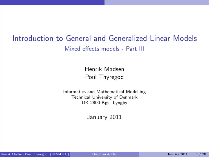
Introduction to General and Generalized Linear Models Mixed effects models - Part III Henrik Madsen Poul Thyregod Informatics and Mathematical Modelling Technical University of Denmark DK-2800 Kgs. Lyngby January 2011 Henrik Madsen Poul Thyregod (IMM-DTU) Chapman & Hall January 2011 1 / 28

This lecture Bayesian Interpretations Posterior distributions for multivariate normal distributions Random effects for multivariate measurements Henrik Madsen Poul Thyregod (IMM-DTU) Chapman & Hall January 2011 2 / 28

Bayesian interpretations Bayesian interpretations In settings where f X ( x ) expresses a so-called “subjective probability distribution” (possibly degenerate), the expression f Y | X = x ( y ) f X ( x ) � f X | Y = y ( x ) = f Y | X = x ( y ) f X ( x ) dx for the conditional distribution of X for given Y = y is termed Bayes’ theorem . In such settings, the distribution f X ( · ) of X is called the prior distribution and the conditional distribution with density function f X | Y = y ( x ) is called the posterior distribution after observation of Y = y . Henrik Madsen Poul Thyregod (IMM-DTU) Chapman & Hall January 2011 3 / 28

Bayesian interpretations Bayesian interpretations Bayes theorem is useful in connection with hierarchical models where the variable X denotes a non-observable state (or parameter) that is associated with the individual experimental object, and Y denotes the observed quantities. In such situations one may often describe the conditional distribution of Y for given state ( X = x ), and one will have observations of the marginal distribution of Y . In general it is not possible to observe the states ( x ), and therefore the distribution f X ( x ) is not observed directly. This situation arises in many contexts such as hidden Markov models (HMM), or state space models, where inference about the state ( X ) can be obtained using the so-called Kalman Filter Henrik Madsen Poul Thyregod (IMM-DTU) Chapman & Hall January 2011 4 / 28

Bayesian interpretations A Bayesian formulation We will discuss the use of Bayes’ theorem in situations where the “prior distribution”, f X ( x ) , has a frequency interpretation. The one-way random effects model may be formulated in a Bayesian framework. We may identify the N ( · , σ 2 u ) -distribution of µ i = µ + U i as the prior distribution . The statistical model for the data is such that for given µ i , are the Y ij ’s independent and distributed like N ( µ i , σ 2 ) . In a Bayesian framework, the conditional distribution of µ i given Y i = y i is termed the posterior distribution for µ i . Henrik Madsen Poul Thyregod (IMM-DTU) Chapman & Hall January 2011 5 / 28

Bayesian interpretations A Bayesian formulation Theorem (The posterior distribution of µ i ) Consider the one-way model with random effects Y ij | µ i ∼ N ( µ i , σ 2 ) µ i ∼ N ( µ, σ 2 u ) where µ , σ 2 and σ 2 u are known. The posterior distribution of µ i after observation of y i 1 , y i 2 , . . . , y in is a normal distribution with mean and variance E[ µ i | Y i = y i ] = µ/σ 2 y i /σ 2 u + n i ¯ = wµ + (1 − w ) y i 1 /σ 2 u + n i /σ 2 1 Var[ µ i | Y i = y i ] = 1 + n σ 2 σ 2 u where 1 1 σ 2 γ = σ 2 u /σ 2 . u w = = with σ 2 + 1 n 1 + nγ σ 2 u Henrik Madsen Poul Thyregod (IMM-DTU) Chapman & Hall January 2011 6 / 28

Bayesian interpretations A Bayesian formulation We observe that the posterior mean is a weighted average of the prior mean µ , and sample result y i with the corresponding precisions (reciprocal variances) as weights. Note that the weights only depend on the signal/noise ratio γ , and not on the numerical values of σ 2 and σ 2 u ; Therefore we may express the posterior mean as y i ] = µ/γ + n i ¯ y i E[ µ i | Y i = ¯ 1 /γ + n i The expression for the posterior variance simplifies, if instead we consider the precision , i.e. the reciprocal variance 1 = 1 + n i σ 2 σ 2 σ 2 post u Henrik Madsen Poul Thyregod (IMM-DTU) Chapman & Hall January 2011 7 / 28

Bayesian interpretations A Bayesian formulation We have that the precision in the posterior distribution is the sum of the precision in the prior distribution and the sampling precision . u /σ 2 and In terms of the signal/noise ratio, γ , with γ prior = σ 2 post /σ 2 we have γ post = σ 2 1 1 = + n i γ post γ prior and µ post = wµ prior + (1 − w )¯ y i with 1 w = 1 + nγ prior in analogy with the BLUP-estimate. Henrik Madsen Poul Thyregod (IMM-DTU) Chapman & Hall January 2011 8 / 28

Bayesian interpretations Estimation under squared error loss The squared error loss function measures the discrepancy between a set of estimates d i ( y ) and the true parameter values µ i , i = 1 , . . . , k and is defind by � k � � � � 2 L ( µ , d ( y )) = d i ( y ) − µ i . i =1 Averaging over the distribution of Y for given value of µ we obtain the risk of using the estimator d ( Y ) when the true parameter is µ � k � � � � 2 R ( µ , d ( . )) = 1 k E Y | µ d i ( y ) − µ i . i =1 Henrik Madsen Poul Thyregod (IMM-DTU) Chapman & Hall January 2011 9 / 28

Bayesian interpretations Estimation under squared error loss Theorem (Risk of the ML-estimator in the one-way model) Let d ML ( Y ) denote the maximum likelihood estimator for µ in the one-way model with fixed effects with µ arbitrary, n � ( Y ) = Y i = 1 d ML Y ij . i n j =1 The risk of this estimator is R ( µ , d ML ) = σ 2 n regardless of the value of µ . Henrik Madsen Poul Thyregod (IMM-DTU) Chapman & Hall January 2011 10 / 28

Bayesian interpretations Estimation under squared error loss Bayes risk for the ML-estimator Introducing the further assumption that µ may be considered as a random variable with the (prior) distribution we may determine Bayes risk of d ML ( · ) under this distribution as r (( µ , γ ) , d ML ) = E µ ( R ( µ , d ML )) Clearly, as R ( µ , d ML ) does not depend on µ we have that the Bayes risk is r (( µ , γ ) , d ML ) = σ 2 n . Henrik Madsen Poul Thyregod (IMM-DTU) Chapman & Hall January 2011 11 / 28

Bayesian interpretations Estimation under squared error loss The Bayes estimator d B ( Y ) is the estimator that minimizes the Bayes risk. d B i ( Y ) = E[ µ i | Y i ] It may be shown that the Bayes risk of this estimator is the posterior variance , σ 2 /n 1 r (( µ , γ ) , d B ) = = 1 + n 1 + 1 / ( nγ ) σ 2 σ 2 u The Bayes risk of the Bayes estimator is less than that of the maximum likelihood estimator. Henrik Madsen Poul Thyregod (IMM-DTU) Chapman & Hall January 2011 12 / 28

Bayesian interpretations The empirical Bayes approach When the parameters ( µ, γ ) in the prior distribution are unknown, one may utilize the whole set of observations Y for estimating µ, γ and σ 2 . We have k � µ = Y .. = 1 SSE σ 2 = � Y i. , � k k ( n − 1) i =1 with SSE ∼ σ 2 χ 2 ( k ( n − 1)) and SSB ∼ σ 2 (1 + nγ ) χ 2 ( k − 1) . As SSE and SSB are independent with � k − 3 � 1 E = SSB σ 2 (1 + nγ ) we find that � � σ 2 � 1 E = 1 + nγ = w. SSB / ( k − 3) Henrik Madsen Poul Thyregod (IMM-DTU) Chapman & Hall January 2011 13 / 28

Bayesian interpretations The empirical Bayes approach Looking at the estimator SSE σ 2 = � k ( n − 1) + 2 and utilize that σ 2 � w = � SSB / ( k − 3) We observe that � w may be expressed by the usual F -test statistic as w = k − 3 k ( n − 1) 1 � k − 1 k ( n − 1) + 2 F Substituting µ and w by the estimates � µ and � w for the posterior mean d B i ( Y ) = E[ µ i | Y i. ] = wµ + (1 − w ) Y i. we obtain the estimator d EB ( Y ) = � w � µ + (1 − � w ) Y i. i The estimator is called an empirical Bayes estimator . Henrik Madsen Poul Thyregod (IMM-DTU) Chapman & Hall January 2011 14 / 28

Bayesian interpretations The empirical Bayes approach Theorem (Bayes risk of the empirical Bayes estimator) Under certain assumptions we have that � � r (( µ , γ ) , d EB ) = 1 2( k − 3) 1 − n { k ( n − 1) + 2 } (1 + nγ ) When k > 3 , then the prior risk for the empirical Bayes estimator d EB is smaller than for the maximum likelihood estimator d ML . The smaller the value of the signal/noise ratio γ , the larger the difference in risk for the two estimators. Henrik Madsen Poul Thyregod (IMM-DTU) Chapman & Hall January 2011 15 / 28

Posterior distributions for multivariate normal distributions Posterior distributions for multivariate normal distributions Theorem (Posterior distribution for multivariate normal distributions) Let Y | µ ∼ N p ( µ , Σ ) and let µ ∼ N p ( m , Σ 0 ) , where Σ and Σ 0 are of full rank, p , say. Then the posterior distribution of µ after observation of Y = y is given by µ | Y = y ∼ N p ( W m + ( I − W ) y , ( I − W ) Σ ) with W = Σ ( Σ 0 + Σ ) − 1 and I − W = Σ 0 ( Σ 0 + Σ ) − 1 Henrik Madsen Poul Thyregod (IMM-DTU) Chapman & Hall January 2011 16 / 28

Posterior distributions for multivariate normal distributions Posterior distributions for multivariate normal distributions If we let Ψ = Σ 0 Σ − 1 denote the generalized ratio between the variation between groups, and the variation within groups, in analogy with the signal to noise ratio, then we can express the weight matrices W and I − W as W = ( I + Ψ ) − 1 and I − W = ( I + Ψ ) − 1 Ψ Henrik Madsen Poul Thyregod (IMM-DTU) Chapman & Hall January 2011 17 / 28